New in 
Bayesian IRF and FEVD analysis
Impulse–response functions (IRFs), dynamic-multiplier functions, and forecast-error variance decompositions (FEVDs) are commonly used to describe the results from multivariate time-series models such as VAR and DSGE models. These models may have many parameters, which may be difficult to interpret. IRFs and other functions combine the effect of multiple parameters into one summary (per time period). For instance, IRFs measure the effect of a shock (change) in one variable such as the inflation rate on a given outcome variable such as the unemployment rate.
In Stata 17, you can perform Bayesian IRF analysis with the new bayesirf command.
Bayesian IRFs (and other functions) are computed from the “exact” posterior distribution of IRFs, which does not rely on the assumption of asymptotic normality. They may also provide more stable estimates for small datasets because they incorporate prior information about the model parameters.
You can produce IRFs and other functions after fitting a Bayesian VAR model by using bayes: var. And you can obtain Bayesian IRFs after fitting Bayesian linear and nonlinear DSGE models by using bayes: dsge and bayes: dsgenl.
bayesirf provides several subcommands for creating, graphing, and tabulating the IRF and related functions. You can create multiple IRF results and combine them in tables and on graphs. You can even include the IRF results from classical frequentist analysis for comparison.
Highlights
- Impulse–response functions
- Dynamic multipliers
- Forecast-error variance decompositions
- Graph and tabulate functions, and save them to current data
- Specify forecast horizon
- Posterior means or medians of functions
- Posterior standard deviations
- Posterior credible intervals
- Create and combine multiple IRF results
Let’s see it work
In Bayesian VAR models, we showed basic Bayesian IRF analysis using the U.S. macrodata, which are quarterly data from the first quarter of 1954 to the fourth quarter of 2010. Here we will show more examples of Bayesian IRF and FEVD analysis.
We want to study the relationships between inflation, output gap, and federal funds rate. In particular, we are interested in the effect of federal funds rate on the other outcomes in the model.
Here are the data.
. webuse usmacro
(Federal Reserve Economic Data - St. Louis Fed)

. tsset

Time variable: date, 1954q3 to 2010q4
        Delta: 1 quarter

. tsline inflation ogap fedfunds

We fit a Bayesian VAR model with three lags. We suppress the output from it here, but you can read more about the command in Bayesian VAR model.
. quietly bayes, rseed(17) saving(bvarsim): var inflation ogap fedfunds, lags(1/3)
The new command bayesirf provides several subcommands for Bayesian IRF and FEVD analysis. Three main ones are bayesirf create, bayesirf graph, and bayesirf table. bayesirf create computes IRFs and other functions and saves them in an IRF dataset, bayesirf graph plots them, and bayesirf table displays them in a table. Other subcommands allow you to combine graphs and tables of multiple functions and manage your IRF results; see [BAYES] bayesirf.
In classical analysis, an IRF (and other functions) is a single function for given response and impulse variables. In Bayesian analysis, we get an entire MCMC sample of IRFs simulated from the posterior distribution. This sample is summarized to produce a single statistic such as posterior mean IRF or posterior median IRF.
We start with creating the IRFs and other functions. We name our IRF results as birf and save them in a Stata dataset birfex.irf.
. bayesirf create birf, set(birfex)
(file birfex.irf created)
(file birfex.irf now active)
(file birfex.irf updated)
Next, we plot the IRF with fedfunds as the impulse variable.
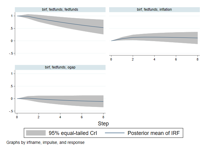
. bayesirf graph irf, impulse(fedfunds)

A shock to the federal funds rate has a positive effect on itself that decreases over time but is still positive after eight quarters. The federal funds rate shock has little effect on the output gap and a small positive effect on inflation that disappears after two quarters.
We can see the results in a table.
. bayesirf table irf, response(ogap) impulse(fedfunds)

Results from birf
| (1) (1) (1) | ||
| Step | irf Lower Upper | |
| 0 | 0 0 0 | |
| 1 | .018505 -.062511 .10086 | |
| 2 | -.013814 -.141146 .116743 | |
| 3 | -.038081 -.193427 .117507 | |
| 4 | -.060205 -.238349 .118354 | |
| 5 | -.078581 -.275435 .120713 | |
| 6 | -.093737 -.307345 .126362 | |
| 7 | -.105821 -.328061 .126226 | |
| 8 | -.115108 -.344162 .127231 | |
We can see the effects of a shock over a longer horizon by specifying more time periods in the step() option of bayesirf create. We replace the current results and additionally save the IRF MCMC sample in birfsim.dta. (We need IRF MCMC results if we want to compute credible intervals other than the default 95% equal-tailed intervals with bayesirf subcommands, which we demonstrate later.)
. bayesirf create birf, set(birfex) step(25) mcmcsaving(birfsim) replace
(file birfex.irf now active)
file birfsim.dta saved.
(file birfex.irf updated)

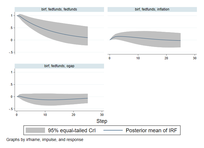
. bayesirf graph irf, impulse(fedfunds)

Adding more time periods allows us to further explore the dynamics of a federal funds rate. A shock on the federal funds rate has a positive effect on itself for the first 14 quarters. We were not able to observe this effect in the previous example with the shorter horizon. Our conclusions about the effect of a federal funds rate on other variables remain the same.
We can look at other functions and plot them side by side by using bayesirf cgraph. Let’s plot orthogonal IRF and FEVD.
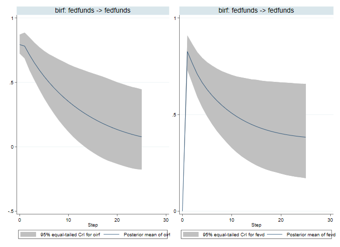
. bayesirf cgraph (birf fedfunds fedfunds oirf) (birf fedfunds fedfunds fevd)

Orthogonal IRFs (OIRFs) describe the impulse response to a one-standard-deviation shock. FEVD measures the fraction of the error variance that is explained by a shock to the federal funds rate. OIRFs support our earlier conclusions based on IRFs. FEVD shows that the shock to fedfunds is prevalent in the first step but then decreases over time.
We can also display multiple results in a table by using bayesirf ctable. For brevity, we show only the first three steps.
. bayesirf ctable (birf fedfunds fedfunds oirf) (birf fedfunds fedfunds fevd), step(3)
| (1) (1) (1) | ||
| Step | oirf Lower Upper | |
| 0 | .793208 .72369 .870942 | |
| 1 | .781637 .686623 .886267 | |
| 2 | .713651 .594886 .848175 | |
| 3 | .652003 .518588 .808557 | |
| (1) (1) (1) | ||
| Step | fevd Lower Upper | |
| 0 | 0 0 0 | |
| 1 | .825878 .731612 .909342 | |
| 2 | .765772 .661851 .86463 | |
| 3 | .709687 .593096 .823202 | |
Instead of the default posterior means and equal-tailed credible intervals, we can report posterior medians and HPD credible intervals. (We can do this because we already saved IRF MCMC results with bayesirf create earlier.)
. bayesirf ctable (birf fedfunds fedfunds oirf) (birf fedfunds fedfunds fevd), step(3) median hpd
| (1) (1) (1) | ||
| Step | oirf Lower Upper | |
| 0 | .79167 .720032 .86681 | |
| 1 | .780219 .686243 .884995 | |
| 2 | .7111 .590842 .842952 | |
| 3 | .648349 .512718 .799466 | |
| (1) (1) (1) | ||
| Step | fevd Lower Upper | |
| 0 | 0 0 0 | |
| 1 | .827376 .737115 .913222 | |
| 2 | .766713 .664094 .865899 | |
| 3 | .710221 .593963 .823788 | |
You can also use the clevel() option to change the default 95% credible level.
After analysis, we remove the files created by bayes: var and bayesirf create if we no longer need them.
. erase bvarsim.dta
. erase birfsim.dta
. erase birfex.irf
