Equations can be dynamic in two senses: lags capture backward-looking behavior, while expected future values capture forward-looking behavior. DSGE models can be used to analyze policies, like the effect of monetary shocks, fiscal shocks, etc.

Bayesian estimation consists of two steps: specifying the DSGE model and specifying priors for the DSGE model parameters.

A small New Keynesian model has an investment–saving (IS) equation that links the output gap to the interest rate, a Phillips curve that links inflation to the output gap, and a Taylor rule that links the interest rate to inflation. In Stata syntax, the model looks like this:

    (   x = F.x - (r - F.p - z)   , unobserved ) ///
    (   p = {beta}*F.p + {kappa}*x             ) ///
    (   r = 1/{delta}*p + m                    ) ///
    ( F.z = {rhoz}*z, state                    ) ///
    ( F.m = {rhom}*m, state                    )

The first equation is an IS curve, the second is a Phillips curve, and the third is a Taylor rule. The fourth equation is an IS shock, and the fifth equation is a Taylor rule monetary shock.

The unobserved option in the IS curve indicates that we treat the output gap as unobserved. We fit the model to data on inflation and the interest rate.
We add a prior specification for each parameter. Many DSGE parameters have interpretations that naturally restrict the range of admissible values. Parameter {beta} in the Phillips curve is a discount rate and must lie between 0 and 1. Parameter {kappa} is a price adjustment parameter, often thought to be small but positive. Parameter {delta} is the inverse of the Taylor rule inflation adjustment coefficient, so it must lie between 0 and 1. In addition to these range restrictions, one might have priors on the probable location of the parameter value. The discount rate is probably around 0.95, the inflation adjustment parameter around 0.2, and the inverse inflation adjustment coefficient around 0.66 (for a Taylor rule coefficient of 1.5). Priors allow you to incorporate that information explicitly in estimation.
Consider the data on the inflation rate and federal funds rate since 1955.

. webuse usmacro2
(Federal Reserve Economic Data - St. Louis Fed, 2017-01-15)

. describe p r


Variable     Storage     Display     Value                          
    name        type      format     label    Variable label        

  p            double     %10.0g              Growth rate of prices (GDPDEF)
  r            double     %10.0g              Federal funds rate (FEDFUNDS)
         
  

. summarize p r


         
 
                                                     
 Variable
 
         Obs         Mean       Std. dev.        Min        Max

       p 
 
        2.44     3.236709       2.281433   -.6681431   11.60957
       r 
 
        2.44     5.035328        3.59569         .07       19.1

Gathering up both the prior specification and the model specification, our estimation command is

. bayes, prior({beta},  beta(95,5))                   ///
         prior({kappa}, beta(30,70))                  ///
         prior({delta}, beta(60,30))                  ///
         prior({rhoz},  beta(10,10))                 ///
         prior({rhom},  beta(10,10))                 ///
         rseed(17) :                                  ///
         dsge (  x = F.x - (r - F.p - z), unobserved) ///
              (  p = {beta}*F.p + {kappa}*x         ) ///
              (  r = 1/{delta}*p + m                ) ///
              (F.z = {rhoz}*z, state                ) ///
              (F.m = {rhom}*m, state                )
note: initial parameter vector set to means of priors.

Burn-in ...
Simulation ...

Model summary
Likelihood:
  p r ~ dsgell({beta},{kappa},{delta},{rhoz},{rhom},{sd(e.z)},{sd(e.m)})

Priors:
             {beta} ~ beta(95,5)
            {kappa} ~ beta(30,70)
            {delta} ~ beta(60,30)
        {rhoz rhom} ~ beta(10,10)
  {sd(e.z) sd(e.m)} ~ igamma(.01,.01)

Bayesian linear DSGE model                     MCMC iterations  =     12,500
Random-walk Metropolis–Hastings sampling       Burn-in          =      2,500
                                               MCMC sample size =     10,000
Sample: 1955q1 thru 2015q4                     Number of obs    =        244
                                               Acceptance rate  =      .2483
                                               Efficiency:  min =    .005767
                                                            avg =     .02115
Log marginal-likelihood = -794.29162                        max =     .03808



       
 
                                                               
       
 
                                                     Equal-tailed
       
 
     Mean     Std. dev.      MCSE     Median     [95% cred. interval]

      beta
 
 .9406005     .0243801    .001984   .9428465     .8869374   .9812481
     kappa
 
  .206337     .0327608    .001679   .2046031     .1470858    .273637
     delta
 
 .5832685     .0404188    .004897   .5835278      .497712   .6607058
      rhoz
 
 .9171911      .015764    .000978   .9170596     .8846393   .9467265
      rhom
 
  .561412     .0296339    .001667   .5621747     .5036024   .6184265
    sd(e.z)
 
 .5280986      .057275    .003639   .5255331     .4217194   .6467684
    sd(e.m)
 
 2.161816     .1585077    .020872   2.141682     1.902066   2.533669

The model summary shows the likelihood model and the prior specifications. The priors for all but the standard deviations are required. In the case of DSGE models, this makes sense because parameters are related to economic theory. For example, the prior for the discount factor {beta} is beta with shape parameters 95 and 5. The standard deviations of the shocks to the state variables z and m were assigned default inverse gamma priors.

The estimation output displays the number of burn-in periods (2,500), the MCMC sample size (10,000), the sample size of the data (244 periods), the sample period (1955q1 through 2015q4), and the acceptance rate and efficiency of the estimation process. The acceptance rate refers to the fraction of MCMC draws that was accepted. Typical values for the Metropolis–Hastings sampler used are 20% to 30%; our acceptance rate is 24%. Efficiency is related to the autocorrelation of the MCMC draws and indicates how quickly the sampler traverses the parameter space. Our average efficiency is 2.1%.

The estimation output displays posterior parameter means, standard deviations, medians, and equal-tailed credible intervals. The posterior mean of {beta} is 0.94, very close to its prior mean of 0.95. The posterior mean of {kappa} is about 0.21, lower than the prior mean of 0.30. The posterior mean for {delta} is 0.58, lower than the prior mean of 0.66. Both shocks are highly persistent, with posterior mean autocorrelation coefficients on z and m of 0.92 and 0.56, respectively. The posterior means of the standard deviations of the shocks are 0.53 for the IS shock z and 2.16 for the Taylor rule monetary shock m.

All of Stata’s Bayesian postestimation features work after bayes: dsge.

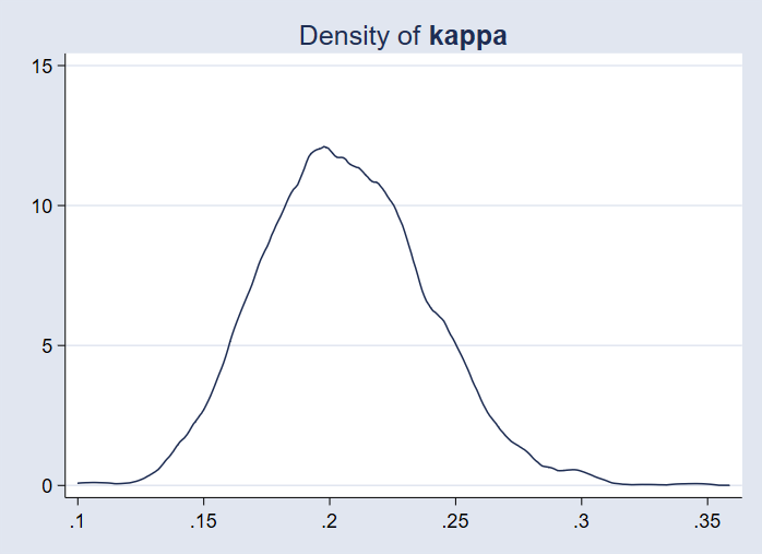
We can plot the posterior density of the prior adjustment parameter {kappa}.

. bayesgraph kdensity {kappa}

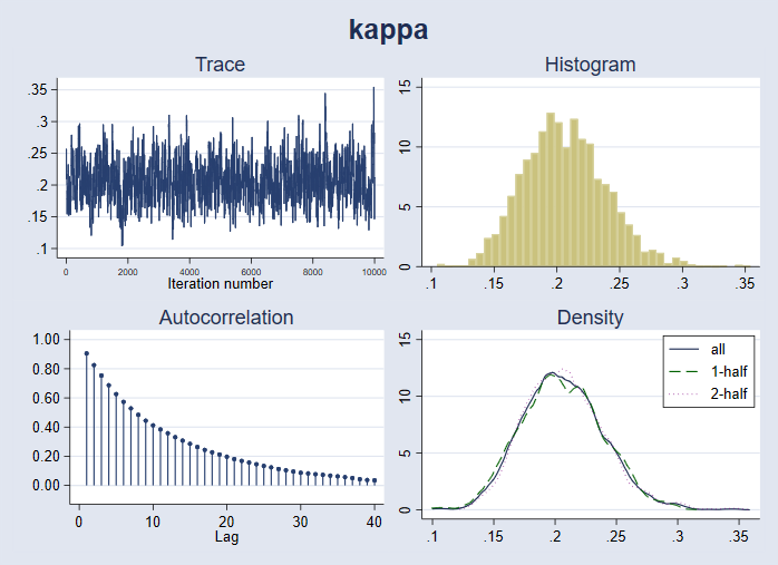
We can plot a full set of diagnostics for {kappa}.

. bayesgraph diagnostics {kappa}

We can add the prior density to the posterior density plot to visually compare the prior and posterior.

. bayesgraph kdensity kappa, addplot(function Prior = betaden(30,70,x), ///
         legend(on label(1 "Posterior")) lcolor(blue))

We can examine posterior densities of functions of model parameters, such as the Taylor rule coefficient 1/{delta}.

. bayesstats summary (1/{delta})

Posterior summary statistics                       MCMC sample size =      10,000

        expr1 : 1/delta



       
 
                                                               
       
 
                                                     Equal-tailed
       
 
     Mean     Std. dev.      MCSE     Median     [95% cred. interval]

      expr1
 
 1.722922     .1225577    .015302   1.713714      1.513533   2.009195

The posterior mean for 1/{delta} is 1.7, higher than the prior mean of 1.5 and indicating a strong response of interest rates to changes in inflation.

We can compute Bayesian impulse–response functions. First, we save the MCMC results to a dataset, nk_mcmc.dta. We can do this during estimation with the saving() option or even after estimation by replaying the bayes command with the saving() option.

. bayes, saving(nk_mcmc.dta, replace)
note: file nk_mcmc.dta not found; file saved.

With the MCMC sample saved, we can construct impulse–response functions with the bayesirf suite. This suite of commands extends irf to accommodate Bayesian estimation and is available after bayes: dsge, bayes: dsgenl, and bayes: var.

. bayesirf set bayes_irfs.irf, replace
(file bayes_irfs.irf created)
(file bayes_irfs.irf now active)

. bayesirf create nk_model
(file bayes_irfs.irf updated)

. bayesirf graph irf, impulse(m) response(x p r m)

The top-left panel shows the response of the monetary state variable m to a shock to itself. The top-right panel shows the response of inflation to the shock: it declines then returns monotonically to steady-state. The bottom-left panel shows the response of the interest rate: it rises. Finally, the bottom-right panel shows the response of the output gap: it falls below 0, indicating a recession. The contractionary monetary shock thus raises the interest rate, reduces inflation, and causes output to decline.

All this and more can be performed with the bayes: dsge command.

Nonlinear DSGE model

The bayes prefix also works with the dsgenl command, which estimates the parameters of nonlinear DSGE models by first-order perturbation.

Next we estimate the parameters of a stochastic growth model. The model has equations for consumption, the real interest rate, GDP, the capital stock, and productivity.

 (1/c     = {beta}*(1/F.c)*(1+F.r-{delta})    )       ///
 (r       = {alpha}*y/k                       )       ///
 (y       = z*k^({alpha})                     )       ///
 (f.k     = y - c + (1-{delta})*k             )       ///
 (ln(f.z) = {rho}*ln(z)                       ) ,     ///
 exostate(z) endostate(k) observed(y) unobserved(c r)

Macroeconomists will recognize these relationships as a consumption Euler equation, a capital demand equation, a production function, a capital accumulation equation, and a law of motion for productivity, respectively.

The parameters have interpretation: {beta} is the discount rate, usually thought to be around 0.95; {alpha} is capital’s share of income, usually thought to be about one-third; {delta} is the depreciation rate, usually 2.5% per quarter; and {rho} is the persistence of the technology shock. Priors are used to bring this information to bear on the estimation.

We estimate the parameters of this model using detrended output. The m1gdp.dta dataset provides the logarithm of output.

. webuse m1gdp, clear

. describe

Contains data from  https://www.stata-press.com/data/r17/m1gdp.dta
 Observations:            223
    Variables:              3                   26 Mar 2020 02:49


Variable     Storage     Display     Value                          
    name        type      format     label    Variable label        

  t               int        %tq              Quarterly time variable
  ln_m1         float      %9.0g              ln(M1) monthly to quarterly by
                                               averaging: M1 is Fred M1SL, Bil
                                               of $ seas adj
  ln_gdp        float      %9.0g              ln(gdpc1) FRED GDP in Bil of 1996
                                               chained $ seas adj

Sorted by: t

The tsfilter command extracts the trend component of output. We use a Hodrick–Prescott filter and then scale the result up by a factor of 100. The resulting scale is such that a value of 1 indicates that GDP is 1% above its trend value.

. tsfilter hp y = ln_gdp

. replace y = 100*y
(222 real changes made)

. tsline y, title("HP-detrended output")

Recessions are associated with a decline in output below trend, while booms are associated with a rise in output above trend.

We proceed with parameter estimation.

. bayes, prior({alpha}, beta(30,70))                ///
         prior({beta},  beta(95,5))                 ///
         prior({delta}, beta(25,900))               ///
         prior({rho},   beta(10, 10))               ///
         rseed(20) dots saving(rbc_mcmc, replace):  ///
         dsgenl (1/c      = {beta}*(1/F.c)*(1+f.r-{delta})    )       ///
                 (r       = {alpha}*y/k                       )       ///
                 (y       = z*k^({alpha})                     )       ///
                 (f.k     = y - c + (1-{delta})*k             )       ///
                 (ln(f.z) = {rho}*ln(z)                       ) ,     ///
                 exostate(z) endostate(k) observed(y) unobserved(c r)
note: initial parameter vector set to means of priors.

Burn-in 2500 aaaaaaaaa1000aaaaaa...2000..... done
Simulation 10000 .........1000.........2000.........3000.........4000.........
5000.........6000.........7000.........8000.........9000.........10000 done

Model summary
Likelihood:
  y ~ dsgell({beta},{delta},{alpha},{rho},{sd(e.z)})

Priors:
     {beta} ~ beta(95,5)
    {delta} ~ beta(25,900)
    {alpha} ~ beta(30,70)
      {rho} ~ beta(10,10)
  {sd(e.z)} ~ igamma(.01,.01)
Bayesian first-order DSGE model                  MCMC iterations  =     12,500
Random-walk Metropolis–Hastings sampling         Burn-in          =      2,500
                                                 MCMC sample size =     10,000
Sample: 1947q1 thru 2002q2                       Number of obs    =        222
                                                 Acceptance rate  =      .2189
                                                 Efficiency:  min =     .02528
                                                              avg =     .04236
Log marginal-likelihood =  -311.7914                          max =     .05567



       
 
                                                               
       
 
                                                   Equal-tailed
       
 
     Mean     Std. dev.      MCSE     Median   [95% cred. interval]

      beta
 
 .9095501     .0392698    .001886   .9133171   .8231531   .9726171
     delta
 
 .0286052     .0054865    .000345      .0284   .0192159   .0404854
     alpha
 
 .2768864     .0451422    .002097   .2738962   .1964999   .3772306
       rho
 
 .7680742      .036755    .001813   .7680699   .6950177   .8412948
    sd(e.z)
 
 .9340691     .0458306    .001943   .9328126   .8502487   1.032548

The prior mean of the discount rate {beta} is 0.95; its posterior mean is little changed at 0.91. The prior mean of the depreciation rate {delta} is 0.025; its posterior mean is little changed at 0.0286. The prior mean of {alpha} is 0.3; its posterior mean is slightly lower at 0.28. Meanwhile, the posterior mean of {rho} is 0.77, much larger than its prior mean of 0.5. The standard deviation of the technology shock is about 1.

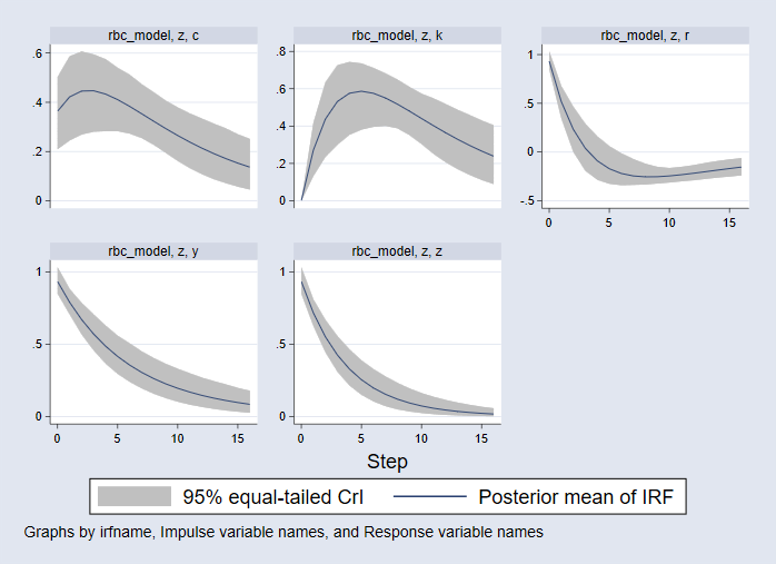
We next compute impulse–response functions to a technology shock.

. bayesirf set bayes_irf2.irf, replace
(file bayes_irf2.irf created)
(file bayes_irf2.irf now active)

. bayesirf create rbc_model, step(16)
(file bayes_irf2.irf updated)

. bayesirf graph irf, impulse(z) byopts(yrescale)

The vertical axis units are in percentage deviations from steady-state. The horizontal axis units are in the same time duration as the data, that is, quarters. We plot 16 steps (4 years) of responses.

• The consumption response is plotted in the top-left panel. Consumption rises on impact and then continues to rise in a hump-shaped pattern before falling back to its steady-state.
• The capital stock response is plotted in the top-middle panel. The capital stock does not move on impact but afterward rises to a peak of 0.6% above its steady-state before declining.
• In the top-right panel, the interest rate rises on impact and then falls; it dips below 0 after four quarters and then returns to its steady-state from below.
• The bottom-left panel plots the response of output; it rises on impact and then falls monotonically back to its steady-state.
• The bottom-middle panel plots the response of technology itself. It, too, rises on impact and then falls monotonically back to its steady-state.

Exact posterior means and credible intervals can be viewed with bayesirf table. Below, we tabulate the response of consumption to a technology shock.

. bayesirf table irf, impulse(z) response(c)

Results from rbc_model



       
 
                                  
       
 
     (1)        (2)         (3)   
  step 
 
     irf       Lower       Upper  

      0
 
 .363699     .209593     .502829
      1
 
 .421867     .245335     .587063
      2
 
 .445802     .269215     .606835
      3
 
 .446962     .280481     .595064
      4
 
 .433453     .282893     .575041
      5
 
 .410962     .282863     .540024
      6
 
 .383436     .272859     .511974
      7
 
 .353574     .254899     .473345
      8
 
 .323189     .227486     .440766
      9
 
 .293459     .195011      .40683
     10
 
 .265119     .162333     .379442
     11
 
 .238595     .133143     .354938
     12
 
 .214099     .108564     .334151
     13
 
   .1917     .087822     .313609
     14
 
 .171372     .071785     .294301
     15
 
 .153031     .057275     .270277
     16
 
 .136556     .045631     .251522

Posterior means reported
95% equal-tailed credible lower and upper bounds reported.
(1) irfname = rbc_model, impulse, = z, and response = c.

After a one-standard-deviation technology shock, consumption rises and peaks at 0.447% above its steady-state value in the third period after the shock.