Launching Version 12.2 of Wolfram Language & Mathematica: 228 New Functions and Much More…
Yet Bigger than Ever Before
When we released Version 12.1 in March of this year, I was pleased to be able to say that with its 182 new functions it was the biggest .1 release we’d ever had. But just nine months later, we’ve got an even bigger .1 release! Version 12.2, launching today, has 228 completely new functions!

We always have a portfolio of development projects going on, with any given project taking anywhere from a few months to more than a decade to complete. And of course it’s a tribute to our whole Wolfram Language technology stack that we’re able to develop so much, so quickly. But Version 12.2 is perhaps all the more impressive for the fact that we didn’t concentrate on its final development until mid-June of this year. Because between March and June we were concentrating on 12.1.1, which was a “polishing release”. No new features, but more than a thousand outstanding bugs fixed (the oldest being a documentation bug from 1993):

How did we design all those new functions and new features that are now in 12.2? It’s a lot of work! And it’s what I personally spend a lot of my time on (along with other “small items” like physics, etc.). But for the past couple of years we’ve done our language design in a very open way—livestreaming our internal design discussions, and getting all sorts of great feedback in real time. So far we’ve recorded about 550 hours—of which Version 12.2 occupied at least 150 hours.
By the way, in addition to all of the fully integrated new functionality in 12.2, there’s also been significant activity in the Wolfram Function Repository—and even since 12.1 was released 534 new, curated functions for all sorts of specialized purposes have been added there.
Biomolecular Sequences: Symbolic DNA, Proteins, etc.
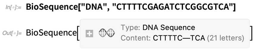
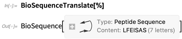
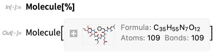
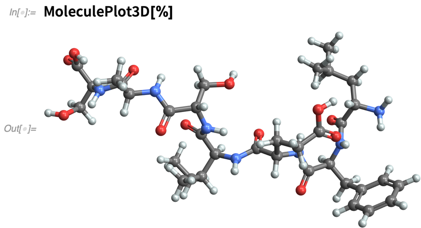
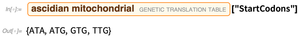
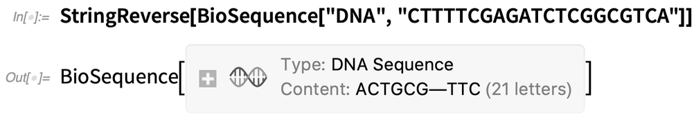
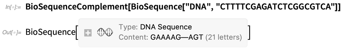
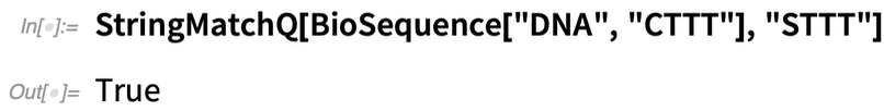
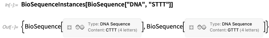
There are so many different things in so many areas in Version 12.2 that it’s hard to know where to start. But let’s talk about a completely new area: bio-sequence computation. Yes, we’ve had gene and protein data in the Wolfram Language for more than a decade. But what’s new in 12.2 is the beginning of the ability to do flexible, general computation with bio sequences. And to do it in a way that fits in with all the chemical computation capabilities we’ve been adding to the Wolfram Language over the past few years.
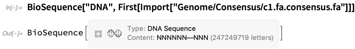
Here’s how we represent a DNA sequence (and, yes, this works with very long sequences too):
 |
 |
 |
 |
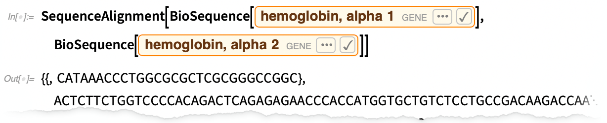
I have to say that I agonized a bit about the “non-universality” of putting the specifics of “our” biology into our core language… but it definitely swayed my thinking that, of course, all our users are (for now) definitively eukaryotes. Needless to say, though, we’re set up to deal with other branches of life too:
 |
 |
 |
 |
 |
 |
 |
 |
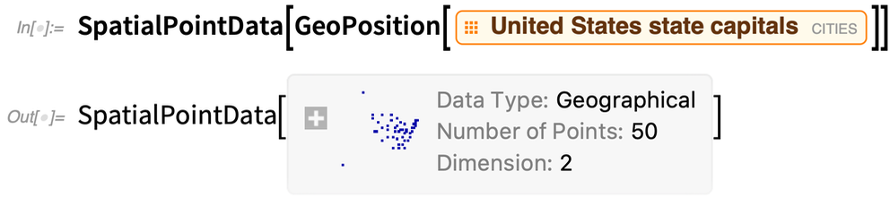
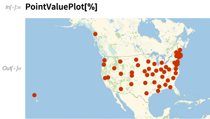
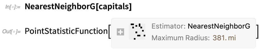
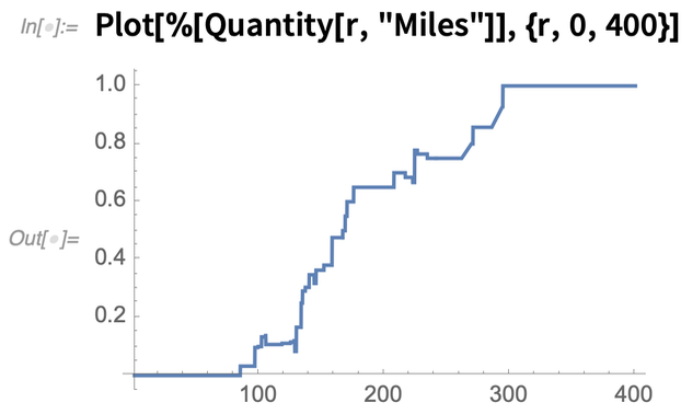
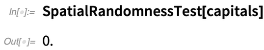
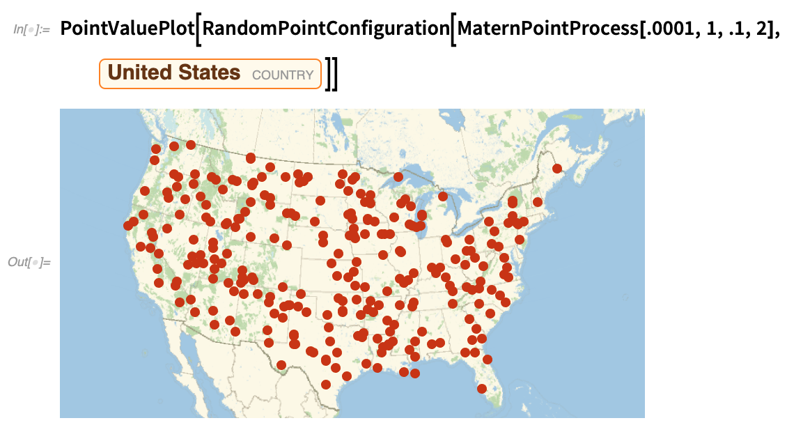
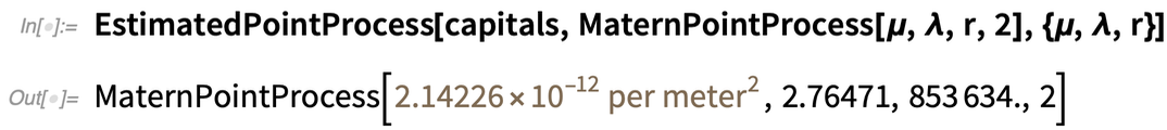
Spatial Statistics & Modeling
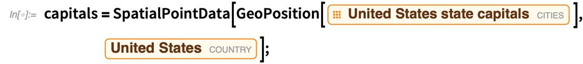
Locations of birds’ nests, gold deposits, houses for sale, defects in a material, galaxies…. These are all examples of spatial point datasets. And in Version 12.2 we now have a broad collection of functions for handling such datasets. Here’s the “spatial point data” for the locations of US state capitals:
 |
 |
 |
 |
 |
 |
 |
 |
 |
 |
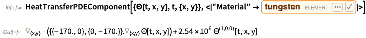
Convenient Real-World PDEs
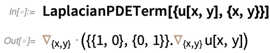
In some ways we’ve been working towards it for 30 years. We first introduced NDSolve back in Version 2.0, and we’ve been steadily enhancing it ever since. But our long-term goal has always been convenient handling of real-world PDEs of the kind that appear throughout high-end engineering. And in Version 12.2 we’ve finally got all the pieces of underlying algorithmic technology to be able to create a truly streamlined PDE-solving experience. OK, so how do you specify a PDE? In the past, it was always done explicitly in terms of particular derivatives, boundary conditions, etc. But most PDEs used for example in engineering consist of higher-level components that “package together” derivatives, boundary conditions, etc. to represent features of physics, materials, etc. The lowest level of our new PDE framework consists of symbolic “terms”, corresponding to common mathematical constructs that appear in real-world PDEs. For example, here’s a 2D “Laplacian term”:
 |
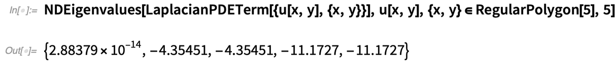 |
 |
 |
 |
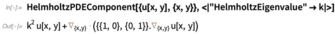 |
 |
 |
 |
What’s basically happening here is that our high-level “physics” description is being “compiled” into explicit “mathematical” PDE structures—like Dirichlet boundary conditions.
OK, so how does all this fit together in a real-life situation? Let me show an example. But first, let me tell a story. Back in 2009 I was having tea with our lead PDE developer. I picked up a teaspoon and asked “When will we be able to model the stresses in this?” Our lead developer explained that there was quite a bit to build to get to that point. Well, I’m excited to say that after 11 years of work, in Version 12.2 we’re there. And to prove it, our lead developer just gave me… a (computational) spoon!
The core of the computation is a 3D diffusion PDE term, with a “diffusion coefficient” given by a rank-4 tensor parametrized by Young’s modulus (here Y) and Poisson ratio (ν):

There are boundary conditions to specify how the spoon is being held, and pushed. Then solving the PDE (which takes just a few seconds) gives the displacement field for the spoon


PDE modeling is a complicated area, and I consider it to be a major achievement that we’ve now managed to “package” it as cleanly as this. But in Version 12.2, in addition to the actual technology of PDE modeling, something else that’s important is a large collection of computational essays about PDE modeling—altogether about 400 pages of detailed explanation and application examples, currently in acoustics, heat transfer and mass transport, but with many other domains to come.
Just Type TEX
The Wolfram Language is all about expressing yourself in precise computational language. But in notebooks you can also express yourself with ordinary text in natural language. But what if you want to display math in there as well? For 25 years we’ve had the infrastructure to do the math display—through our box language. But the only convenient way to enter the math is through Wolfram Language math constructs—that in some sense have to have computational meaning.
But what about “math” that’s “for human eyes only”? That has a certain visual layout that you want to specify, but that doesn’t necessarily have any particular underlying computational meaning that’s been defined? Well, for many decades there’s been a good way to specify such math, thanks to my friend Don Knuth: just use TEX. And in Version 12.2 we’re now supporting direct entry of TEX math into Wolfram Notebooks, both on the desktop and in the cloud. Underneath, the TEX is being turned into our box representation, so it structurally interoperates with everything else. But you can just enter it—and edit it—as TEX.
The interface is very much like the ctrl+= interface for Wolfram|Alpha-style natural language input. But for TEX (in a nod to standard TEX delimiters), it’s ctrl>+$.
Type ctrl+$ and you get a TEX input box. When you’ve finished the TEX, just hit ctrl and it’ll be rendered:


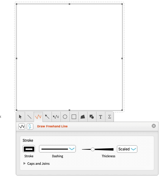
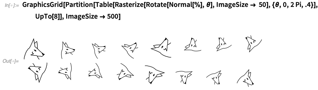
Just Draw Anything
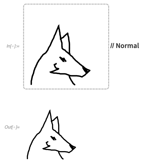
Type Canvas[] and you’ll get a blank canvas to draw whatever you want:
![Canvas[]](https://sciexperts.com/wp-content/uploads/2022/04/just-draw-anything-canvas-02.png)
We’ve worked hard to make the drawing tools as ergonomic as possible.
Applying Normal gives you graphics that you can then use or manipulate:
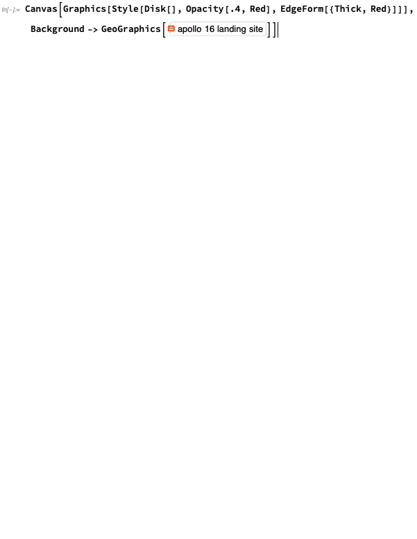
When you create a canvas, it can have any graphic as initial content—and it can have any background you want:
 It’s another molecule now:

The Never-Ending Math Story
Math has been a core use case for the Wolfram Language (and Mathematica) since the beginning. And it’s been very satisfying over the past third of a century to see how much math we’ve been able to make computational. But the more we do, the more we realize is possible, and the further we can go. It’s become in a sense routine for us. There’ll be some area of math that people have been doing by hand or piecemeal forever. And we’ll figure out: yes, we can make an algorithm for that! We can use the giant tower of capabilities we’ve built over all these years to systematize and automate yet more mathematics; to make yet more math computationally accessible to anyone. And so it has been with Version 12.2. A whole collection of pieces of “math progress”. Let’s start with something rather cut and dried: special functions. In a sense, every special function is an encapsulation of a certain nugget of mathematics: a way of defining computations and properties for a particular type of mathematical problem or system. Starting from Mathematica 1.0 we’ve achieved excellent coverage of special functions, steadily expanding to more and more complicated functions. And in Version 12.2 we’ve got another class of functions: the Lamé functions. Lamé functions are part of the complicated world of handling ellipsoidal coordinates; they appear as solutions to the Laplace equation in an ellipsoid. And now we can evaluate them, expand them, transform them, and do all the other kinds of things that are involved in integrating a function into our language: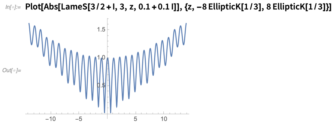
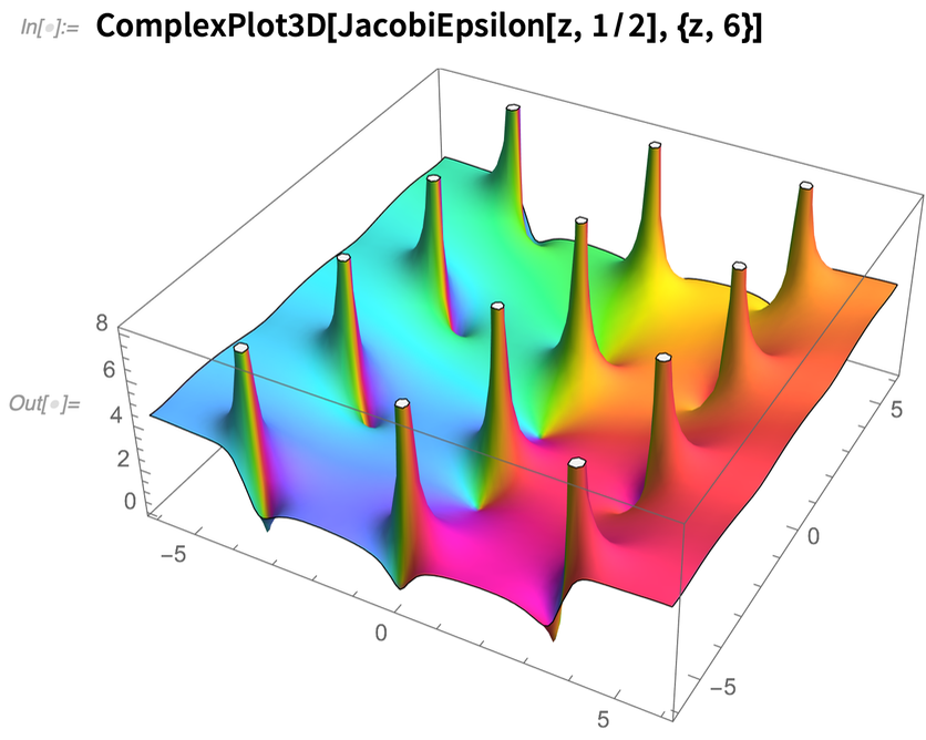
 Also in Version 12.2 we’ve done a lot on elliptic functions—dramatically speeding up their numerical evaluation and inventing algorithms doing this efficiently at arbitrary precision. We’ve also introduced some new elliptic functions, like JacobiEpsilon—which provides a generalization of EllipticE that avoids branch cuts and maintains the analytic structure of elliptic integrals:
 We’ve been able to do many symbolic Laplace and inverse Laplace transforms for a couple of decades. But in Version 12.2 we’ve solved the subtle problem of using contour integration to do inverse Laplace transforms. It’s a story of knowing enough about the structure of functions in the complex plane to avoid branch cuts and other nasty singularities. A typical result effectively sums over an infinite number of poles:
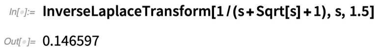
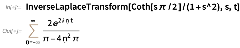 And between contour integration and other methods we’ve also added numerical inverse Laplace transforms. It all looks easy in the end, but there’s a lot of complicated algorithmic work needed to achieve this:
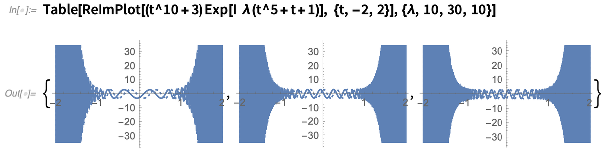
 Another new algorithm made possible by finer “function understanding” has to do with asymptotic expansion of integrals. Here’s a complex function that becomes increasingly wiggly as λ increases:
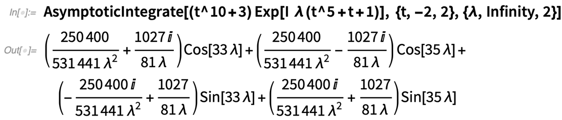
 And here’s the asymptotic expansion for λ→∞:
Tell Me about That Function
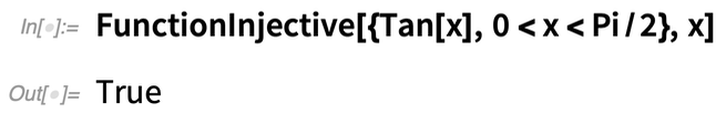
It’s a very common calculus exercise to determine, for example, whether a particular function is injective. And it’s pretty straightforward to do this in easy cases. But a big step forward in Version 12.2 is that we can now systematically figure out these kinds of global properties of functions—not just in easy cases, but also in very hard cases. Often there are whole networks of theorems that depend on functions having such-and-such a property. Well, now we can automatically determine whether a particular function has that property, and so whether the theorems hold for it. And that means that we can create systematic algorithms that automatically use the theorems when they apply. Here’s an example. Is Tan[x] injective? Not globally: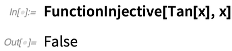 But over an interval, yes:
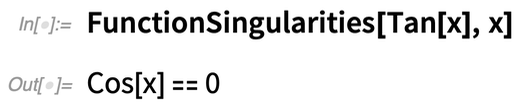
 What about the singularities of Tan[x]? This gives a description of the set:
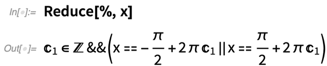
 You can get explicit values with Reduce:
 So far, fairly straightforward. But things quickly get more complicated:
 And there are more sophisticated properties you can ask about as well:
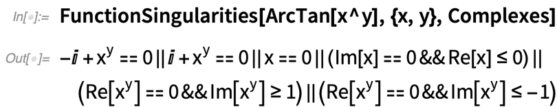
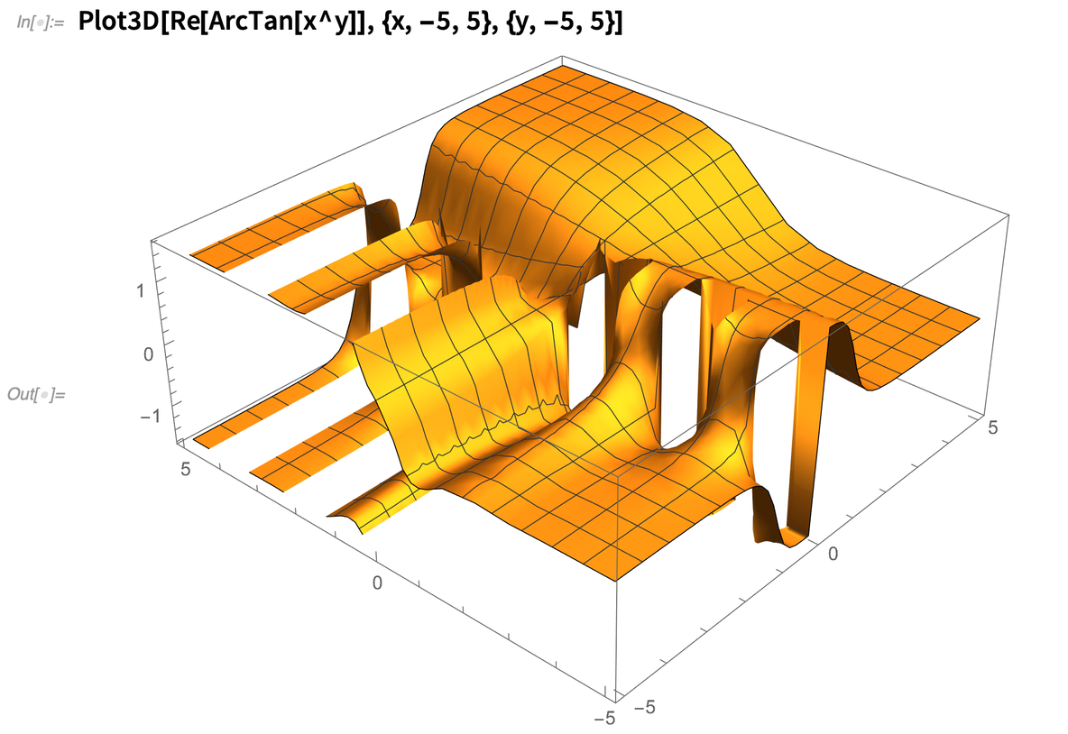
 We’ve internally used various kinds of function-testing properties for a long time. But with Version 12.2 function properties are much more complete and fully exposed for anyone to use. Want to know if you can interchange the order of two limits? Check FunctionSingularities. Want to know if you can do a multivariate change of variables in an integral? Check FunctionInjective.
And, yes, even in Plot3D we’re routinely using FunctionSingularities to figure out what’s going on:
We’ve internally used various kinds of function-testing properties for a long time. But with Version 12.2 function properties are much more complete and fully exposed for anyone to use. Want to know if you can interchange the order of two limits? Check FunctionSingularities. Want to know if you can do a multivariate change of variables in an integral? Check FunctionInjective.
And, yes, even in Plot3D we’re routinely using FunctionSingularities to figure out what’s going on:
Mainstreaming Video
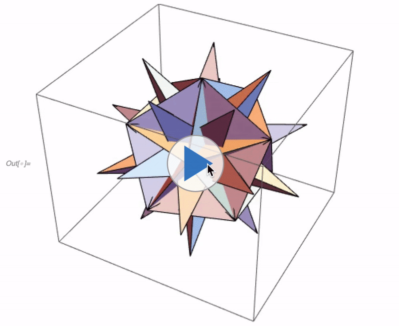
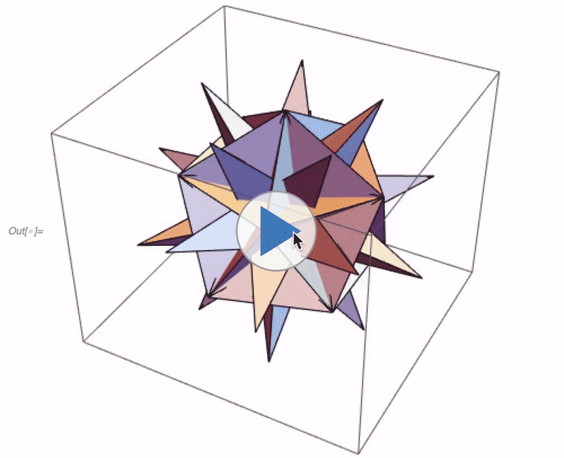
In Version 12.1 we began the process of introducing video as a built-in feature of the Wolfram Language. Version 12.2 continues that process. In 12.1 we could only handle video in desktop notebooks; now it’s extended to cloud notebooks—so when you generate a video in Wolfram Language it’s immediately deployable to the cloud. A major new video feature in 12.2 is VideoGenerator. Provide a function that makes images (and/or audio), and VideoGenerator will generate a video from them (here a 4-second video):
 To add a sound track, we can just use VideoCombine:
 But the real power of the Wolfram Language comes in systematically applying arbitrary functions to videos. VideoMap lets you apply a function to a video to get another video. For example, we could progressively blur the video we just made:
 There are also two new functions for analyzing videos—VideoMapList and VideoMapTimeSeries—which respectively generate a list and a time series by applying a function to the frames in a video, and to its audio track.
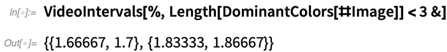
Another new function—highly relevant for video processing and video editing—is VideoIntervals, which determines the time intervals over which any given criterion applies in a video:
There are also two new functions for analyzing videos—VideoMapList and VideoMapTimeSeries—which respectively generate a list and a time series by applying a function to the frames in a video, and to its audio track.
Another new function—highly relevant for video processing and video editing—is VideoIntervals, which determines the time intervals over which any given criterion applies in a video:
 Now, for example, we can delete those intervals in the video:
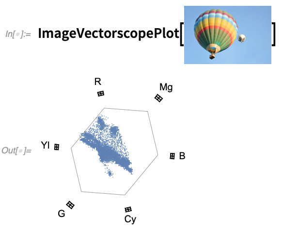
 A common operation in the practical handling of videos is transcoding. And in Version 12.2 the function VideoTranscode lets you convert a video among any of the over 300 containers and codecs that we support. By the way, 12.2 also has new functions ImageWaveformPlot and ImageVectorscopePlot that are commonly used in video color correction:
 One of the main technical issues in handling video is dealing with the large amount of data in a typical video. In Version 12.2 there’s now finer control over where that data is stored. The option GeneratedAssetLocation (with default $GeneratedAssetLocation) lets you pick between different files, directories, local object stores, etc.
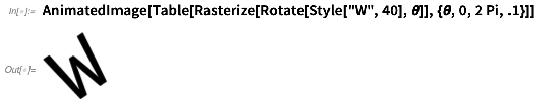
But there’s also a new function in Version 12.2 for handling “lightweight video”, in the form of AnimatedImage. AnimatedImage simply takes a list of images and produces an animation that immediately plays in your notebook—and has everything directly stored in your notebook.
One of the main technical issues in handling video is dealing with the large amount of data in a typical video. In Version 12.2 there’s now finer control over where that data is stored. The option GeneratedAssetLocation (with default $GeneratedAssetLocation) lets you pick between different files, directories, local object stores, etc.
But there’s also a new function in Version 12.2 for handling “lightweight video”, in the form of AnimatedImage. AnimatedImage simply takes a list of images and produces an animation that immediately plays in your notebook—and has everything directly stored in your notebook.
Big Computations? Send Them to a Cloud Provider!
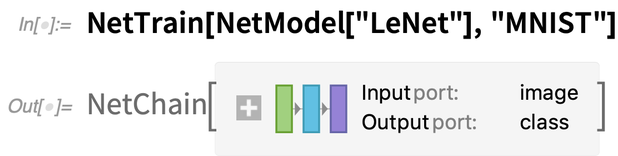
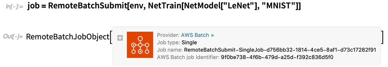
It comes up quite frequently for me—especially given our Physics Project. I’ve got a big computation I’d like to do, but I don’t want to (or can’t) do it on my computer. And instead what I’d like to do is run it as a batch job in the cloud. This has been possible in principle for as long as cloud computation providers have been around. But it’s been very involved and difficult. Well, now, in Version 12.2 it’s finally easy. Given any piece of Wolfram Language code, you can just use RemoteBatchSubmit to send it to be run as a batch job in the cloud. There’s a little bit of setup required on the batch computation provider side. First, you have to have an account with an appropriate provider—and initially we’re supporting AWS Batch and Charity Engine. Then you have to configure things with that provider (and we’ve got workflows that describe how to do that). But as soon as that’s done, you’ll get a remote batch submission environment that’s basically all you need to start submitting batch jobs: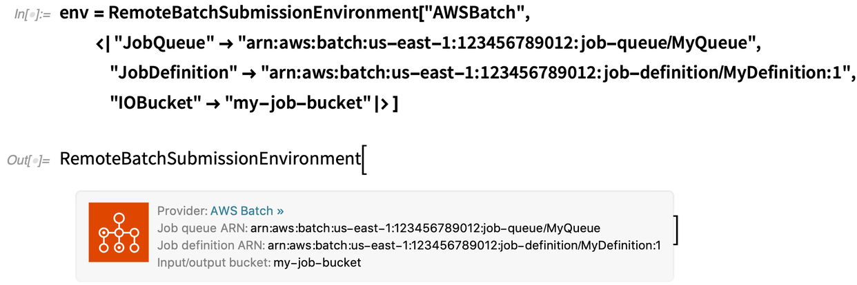 OK, so what would be involved, say, in submitting a neural net training? Here’s how I would run it locally on my machine (and, yes, this is a very simple example):
 And here’s the minimal way I would send it to run on AWS Batch:
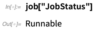
 I get back an object that represents my remote batch job—that I can query to find out what’s happened with my job. At first it’ll just tell me that my job is “runnable”:
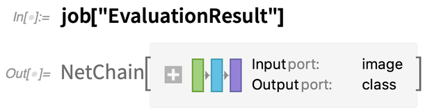
 Later on, it’ll say that it’s “starting”, then “running”, then (if all goes well) “succeeded”. And once the job is finished, you can get back the result like this:
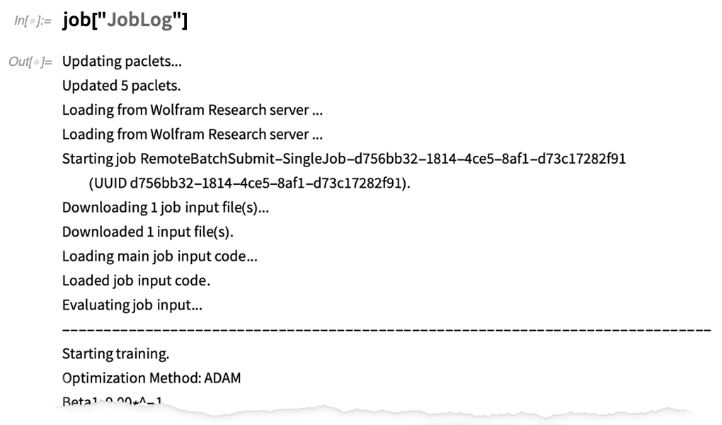
 There’s lots of detail you can retrieve about what actually happened. Like here’s the beginning of the raw job log:
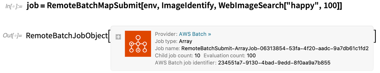
 But the real point of running your computations remotely in a cloud is that they can potentially be bigger and crunchier than the ones you can run on your own machines. Here’s how we could run the same computation as above, but now requesting the use of a GPU:
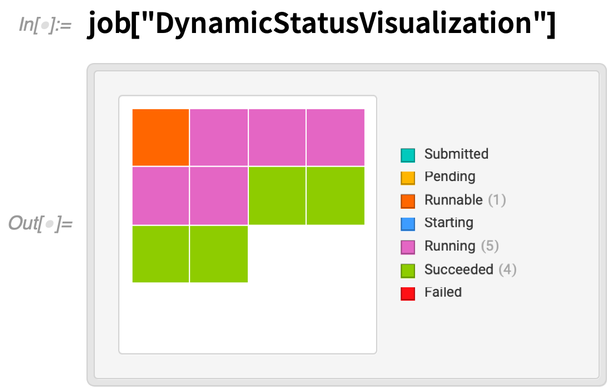
 While it’s running, we can get a dynamic display of the status of each part of the job:
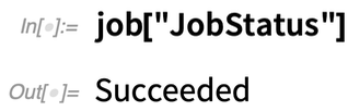
 About 5 minutes later, the job is finished:
 RemoteBatchSubmit and RemoteBatchMapSubmit give you high-level access to cloud compute services for general batch computation. But in Version 12.2 there is also a direct lower-level interface available, for example for AWS.
Connect to AWS:
RemoteBatchSubmit and RemoteBatchMapSubmit give you high-level access to cloud compute services for general batch computation. But in Version 12.2 there is also a direct lower-level interface available, for example for AWS.
Connect to AWS:
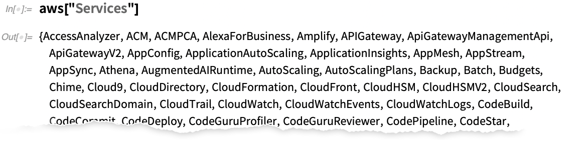
 Once you’ve authenticated, you can see all the services that are available:
 This gives a handle to the Amazon Translate service:
 Now you can use this to call the service:
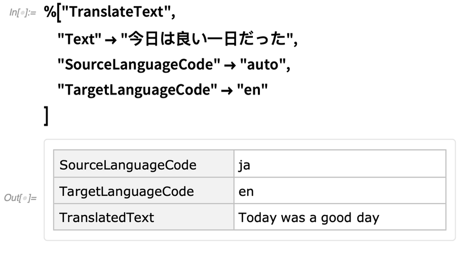 Of course, you can always do language translation directly through the Wolfram Language too:

Can You Make a 10-Dimensional Plot?
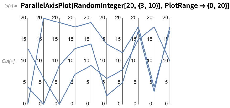
It’s straightforward to plot data that involves one, two or three dimensions. For a few dimensions above that, you can use colors or other styling. But by the time you’re dealing with ten dimensions, that breaks down. And if you’ve got a lot of data in 10D, for example, then you’re probably going to have to use something like DimensionReduce to try to tease out “interesting features”. But if you’re just dealing with a few “data points”, there are other ways to visualize things like 10-dimensional data. And in Version 12.2 we’re introducing several functions for doing this. As a first example, let’s look at ParallelAxisPlot. The idea here is that every “dimension” is plotted on a “separate axis”. For a single point it’s not that exciting: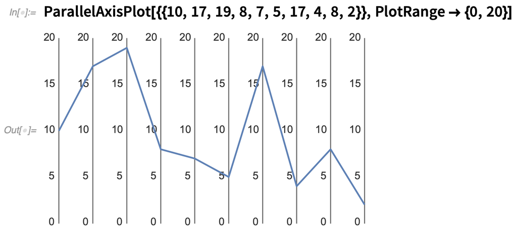 Here’s what happens if we plot three random “10D data points”:
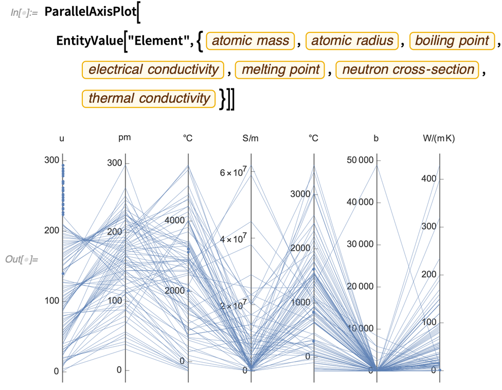
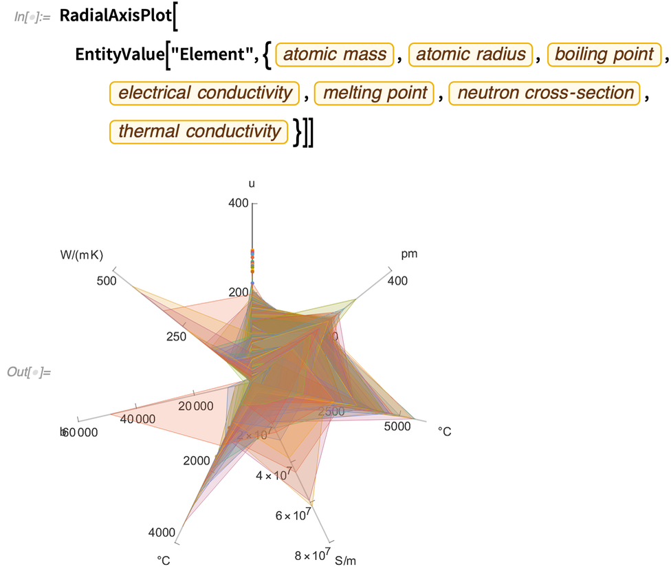
 But one of the important features of ParallelAxisPlot is that by default it automatically determines the scale on each axis, so there’s no need for the axes to be representing similar kinds of things. So, for example, here are 7 completely different quantities plotted for all the chemical elements:
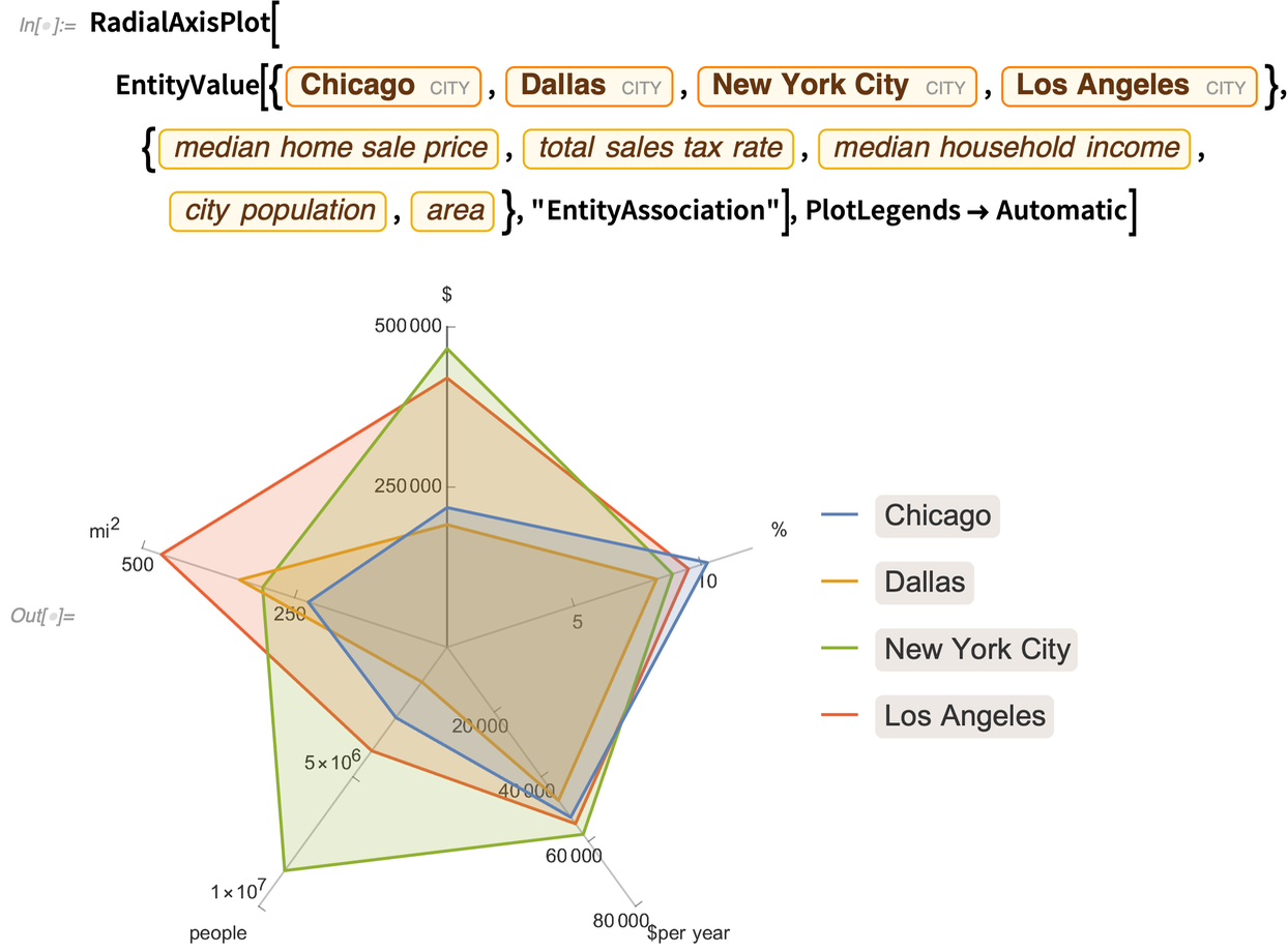
 Different kinds of high-dimensional data do best on different kinds of plots. Another new type of plot in Version 12.2 is RadialAxisPlot. (This type of plot also goes by names like radar plot, spider plot and star plot.)
RadialAxisPlot plots each dimension in a different direction:
Different kinds of high-dimensional data do best on different kinds of plots. Another new type of plot in Version 12.2 is RadialAxisPlot. (This type of plot also goes by names like radar plot, spider plot and star plot.)
RadialAxisPlot plots each dimension in a different direction:
 It’s typically most informative when there aren’t too many data points:
3D Array Plots
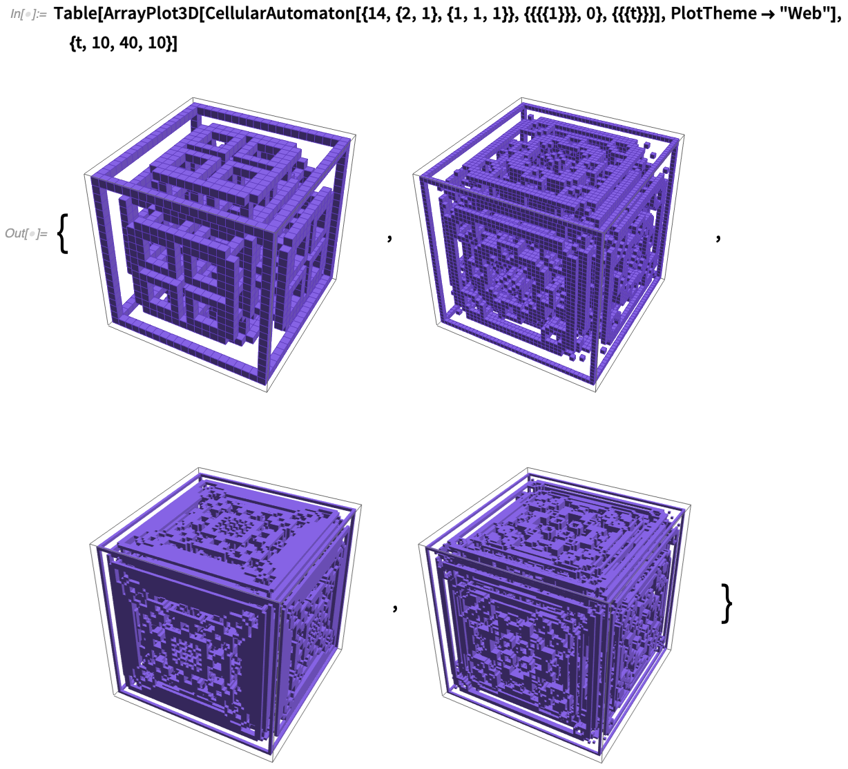
Back in 1984 I used a Cray supercomputer to make 3D pictures of 2D cellular automata evolving in time (yes, captured on 35 mm slides):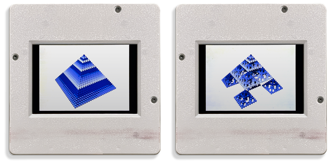 I’ve been waiting for 36 years to have a really streamlined way to reproduce these. And now finally in Version 12.2 we have it: ArrayPlot3D. Already in 2012 we introduced Image3D to represent and display 3D images composed of 3D voxels with specified colors and opacities. But its emphasis is on “radiology-style” work, in which there’s a certain assumption of continuity between voxels. And if you’ve really got a discrete array of discrete data (as in cellular automata) that won’t lead to crisp results.
And here it is, for a slightly more elaborate case of a 3D cellular automaton:
I’ve been waiting for 36 years to have a really streamlined way to reproduce these. And now finally in Version 12.2 we have it: ArrayPlot3D. Already in 2012 we introduced Image3D to represent and display 3D images composed of 3D voxels with specified colors and opacities. But its emphasis is on “radiology-style” work, in which there’s a certain assumption of continuity between voxels. And if you’ve really got a discrete array of discrete data (as in cellular automata) that won’t lead to crisp results.
And here it is, for a slightly more elaborate case of a 3D cellular automaton:
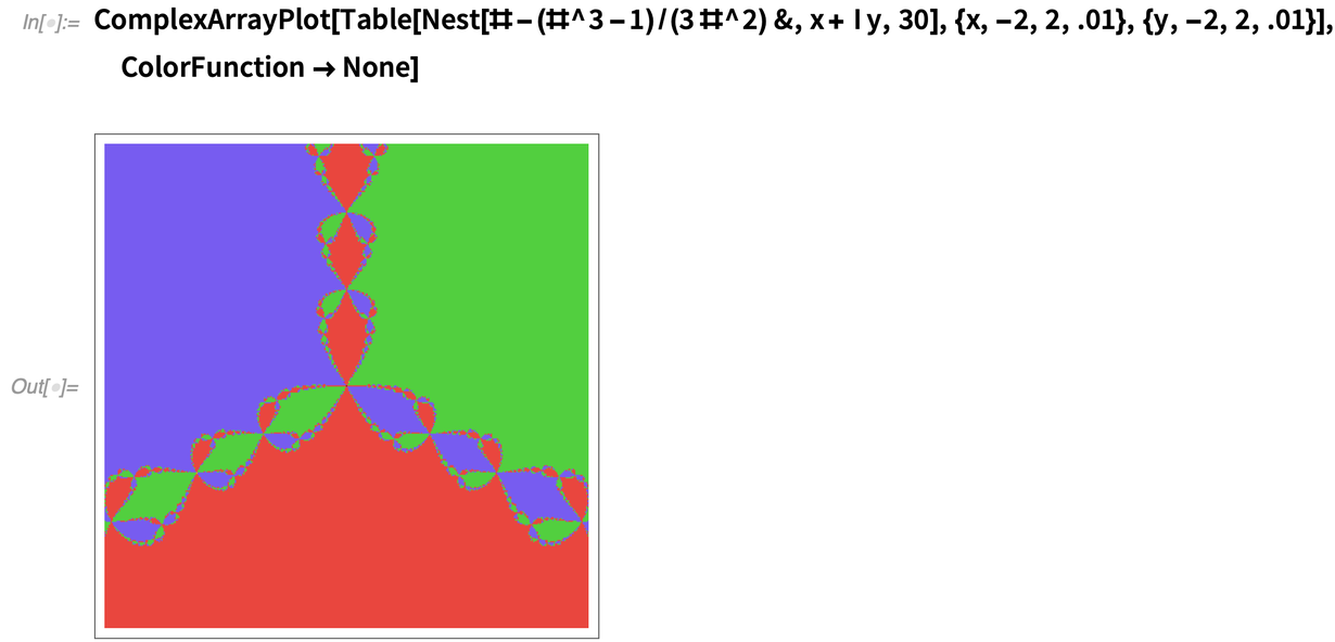
 Another new ArrayPlot-family function in 12.2 is ComplexArrayPlot, here applied to an array of values from Newton’s method:
Advancing the Computational Aesthetics of Visualization
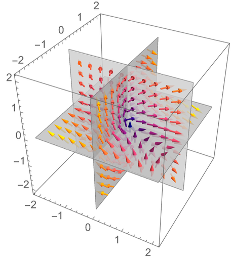
One of our objectives in Wolfram Language is to have visualizations that just “automatically look good”—because they’ve got algorithms and heuristics that effectively implement good computational aesthetics. In Version 12.2 we’ve tuned up the computational aesthetics for a variety of types of visualization. For example, in 12.1 this is what a SliceVectorPlot3D looked like by default: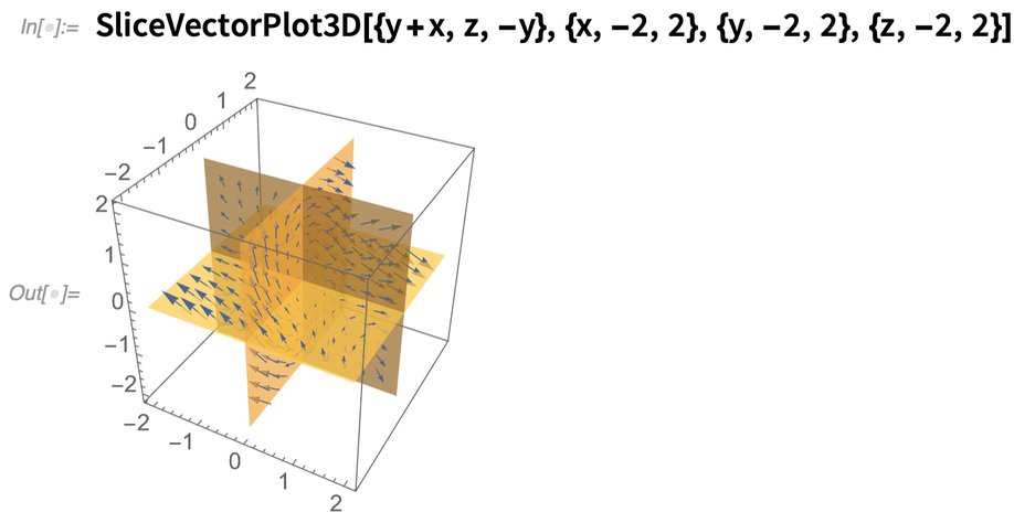 Now it looks like this:
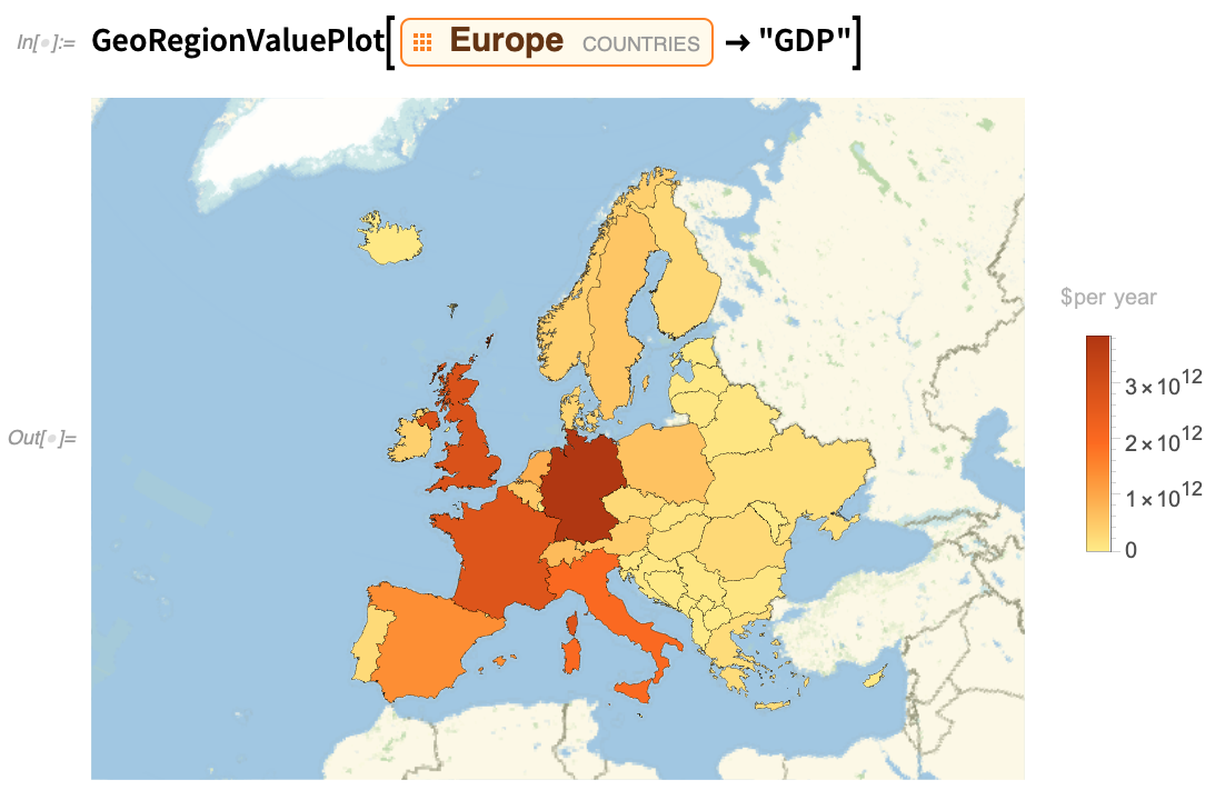
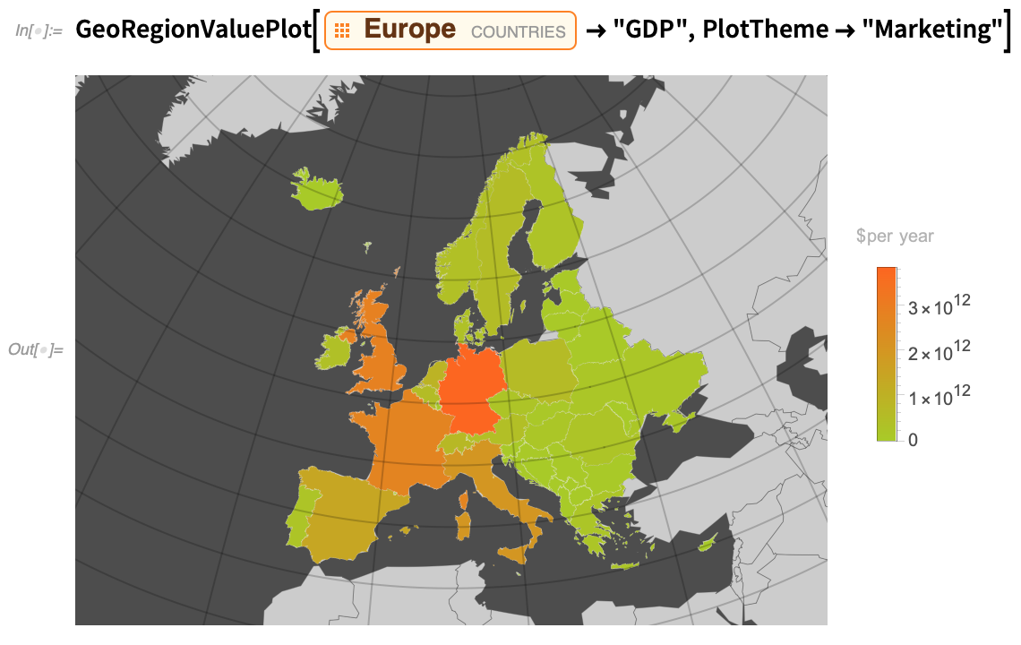
 Since Version 10, we’ve also been making increasing use of our PlotTheme option, to “bank switch” detailed options to make visualizations that are suitable for different purposes, and meet different aesthetic goals. So for example in Version 12.2 we’ve added plot themes to GeoRegionValuePlot. Here’s an example of the default (which has been updated, by the way):
 And here it is with the “Marketing” plot theme:
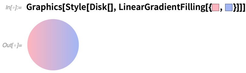
 Another thing in Version 12.2 is the addition of new primitives and new “raw material” for creating aesthetic visual effects. In Version 12.1 we introduced things like HatchFilling for cross-hatching. In Version 12.2 we now also have LinearGradientFilling:
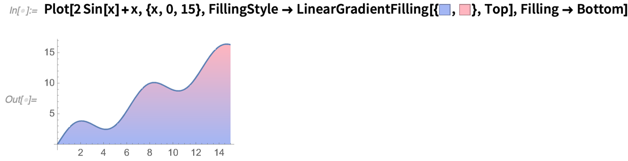
 And we can now add this kind of effect to the filling in a plot:
 To be even more stylish, one can plot random points using the new ConicGradientFilling:

Making Code Just a Bit More Beautiful
A core goal of the Wolfram Language is to define a coherent computational language that can readily be understood by both computers and humans. We (and I in particular!) put a lot of effort into the design of the language, and into things like picking the right names for functions. But in making the language as easy to read as possible, it’s also important to streamline its “non-verbal” or syntactic aspects. For function names, we’re basically leveraging people’s understanding of words in natural language. For syntactic structure, we want to leverage people’s “ambient understanding”, for example, from areas like math. More than a decade ago we introduced as a way to specify Function functions, so instead of writing
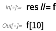
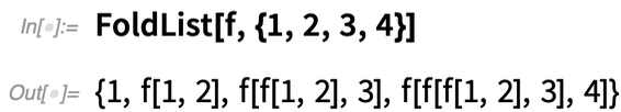
 We’re always on the lookout for repeated “lumps of computation” that we can “package” into functions with “easy-to-understand names”. And in Version 12.2 we have a couple of new such functions: FoldWhile and FoldWhileList. FoldList normally just takes a list and “folds” each successive element into the result it’s building up—until it gets to the end of the list:
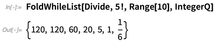
 But what if you want to “stop early”? FoldWhileList lets you do that. So here we’re successively dividing by 1, 2, 3, …, stopping when the result isn’t an integer anymore:
More Array Gymnastics: Column Operations and Their Generalizations
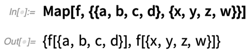
Let’s say you’ve got an array, like: Map lets you map a function over the “rows” of this array:
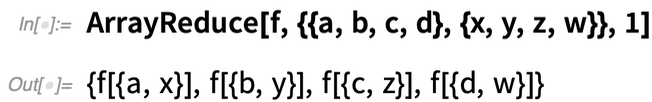
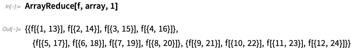
 But what if you want to operate on the “columns” of the array, effectively “reducing out” the first dimension of the array? In Version 12.2 the function ArrayReduce lets you do this:
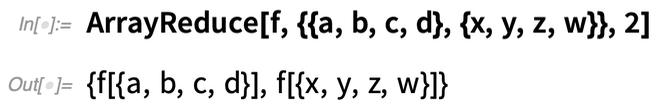
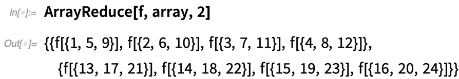
 Here’s what happens if instead we tell ArrayReduce to “reduce out” the second dimension of the array:
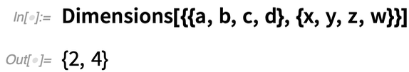
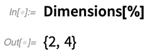
 What’s really going on here? The array has dimensions 2×4:
 ArrayReduce[f, ..., 1] “reduces out” the first dimension, leaving an array with dimensions {4}.
ArrayReduce[f, ..., 2] reduces out the second dimension, leaving an array with dimensions {2}.
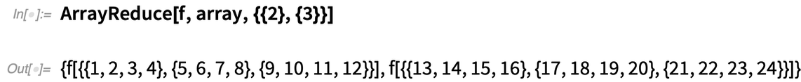
Let’s look at a slightly bigger case—a 2×3×4 array:
ArrayReduce[f, ..., 1] “reduces out” the first dimension, leaving an array with dimensions {4}.
ArrayReduce[f, ..., 2] reduces out the second dimension, leaving an array with dimensions {2}.
Let’s look at a slightly bigger case—a 2×3×4 array:
 This now eliminates the “first dimension”, leaving a 3×4 array:
 This, on the other hand, eliminates the “second dimension”, leaving a 2×4 array:
 Why is this useful? One example is when you have arrays of data where different dimensions correspond to different attributes, and then you want to “ignore” a particular attribute, and aggregate the data with respect to it. Let’s say that the attribute you want to ignore is at level n in your array. Then all you do to “ignore” it is to use ArrayReduce[f, ..., n], where f is the function that aggregates values (often something like Total or Mean).
You can achieve the same results as ArrayReduce by appropriate sequences of Transpose, Apply, etc. But it’s quite messy, and ArrayReduce provides an elegant “packaging” of these kinds of array operations.
Why is this useful? One example is when you have arrays of data where different dimensions correspond to different attributes, and then you want to “ignore” a particular attribute, and aggregate the data with respect to it. Let’s say that the attribute you want to ignore is at level n in your array. Then all you do to “ignore” it is to use ArrayReduce[f, ..., n], where f is the function that aggregates values (often something like Total or Mean).
You can achieve the same results as ArrayReduce by appropriate sequences of Transpose, Apply, etc. But it’s quite messy, and ArrayReduce provides an elegant “packaging” of these kinds of array operations.

 At the simplest level, ArrayReduce is a convenient way to apply functions “columnwise” on arrays. But in full generality it’s a way to apply functions to subarrays with arbitrary indices. And if you’re thinking in terms of tensors, ArrayReduce is a generalization of contraction, in which more than two indices can be involved, and elements can be “flattened” before the operation (which doesn’t have to be summation) is applied.
Watch Your Code Run: More in the Echo Family
It’s an old adage in debugging code: “put in a print statement”. But it’s more elegant in the Wolfram Language, thanks particularly to Echo. It’s a simple idea: Echo[expr] “echoes” (i.e. prints) the value of expr, but then returns that value. So the result is that you can put Echo anywhere into your code (often as Echo@…) without affecting what your code does. In Version 12.2 there are some new functions that follow the “Echo” pattern. A first example is EchoLabel, which just adds a label to what’s echoed: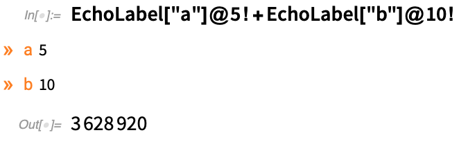 Aficionados might wonder why EchoLabel is needed. After all, Echo itself allows a second argument that can specify a label. The answer—and yes, it’s a mildly subtle piece of language design—is that if one’s going to just insert Echo as a function to apply (say with @), then it can only have one argument, so no label. EchoLabel is set up to have the operator form EchoLabel[label] so that EchoLabel[label][expr] is equivalent to Echo[expr,label].
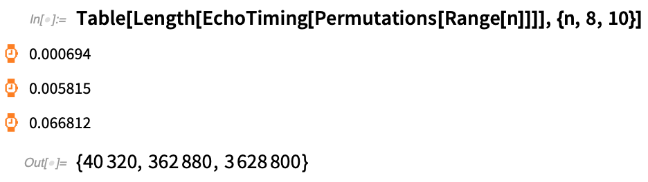
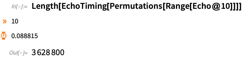
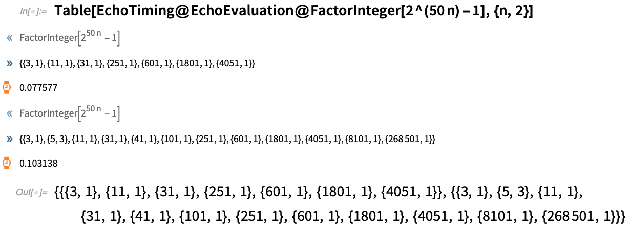
Another new “echo function” in 12.2 is EchoTiming, which displays the timing (in seconds) of whatever it evaluates:
Aficionados might wonder why EchoLabel is needed. After all, Echo itself allows a second argument that can specify a label. The answer—and yes, it’s a mildly subtle piece of language design—is that if one’s going to just insert Echo as a function to apply (say with @), then it can only have one argument, so no label. EchoLabel is set up to have the operator form EchoLabel[label] so that EchoLabel[label][expr] is equivalent to Echo[expr,label].
Another new “echo function” in 12.2 is EchoTiming, which displays the timing (in seconds) of whatever it evaluates:
 It’s often helpful to use both Echo and EchoTiming:
 And, by the way, if you always want to print evaluation time (just like Mathematica 1.0 did by default 32 years ago) you can always globally set $Pre=EchoTiming.
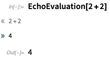
Another new “echo function” in 12.2 is EchoEvaluation which echoes the “before” and “after” for an evaluation:
And, by the way, if you always want to print evaluation time (just like Mathematica 1.0 did by default 32 years ago) you can always globally set $Pre=EchoTiming.
Another new “echo function” in 12.2 is EchoEvaluation which echoes the “before” and “after” for an evaluation:
 You might wonder what happens with nested EchoEvaluation’s. Here’s an example:
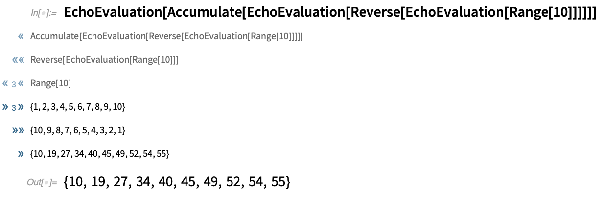 By the way, it’s quite common to want to use both EchoTiming and EchoEvaluation:
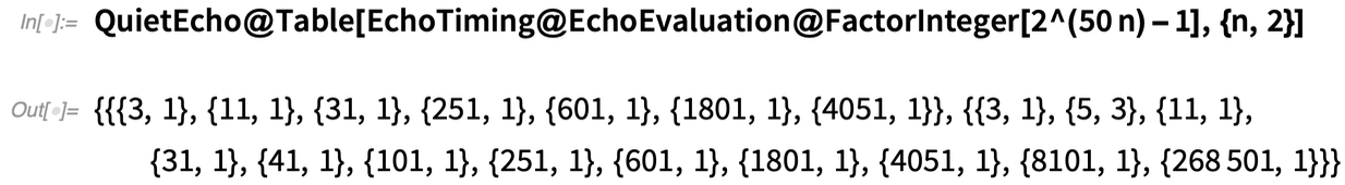
 Finally, if you want to leave echo functions in your code, but want your code to “run quiet”, you can use the new QuietEcho to “quiet” all the echoes (like Quiet “quiets” messages):
Making Code Just a Bit More Beautiful
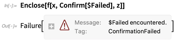
Did something go wrong inside your program? And if so, what should the program do? It can be possible to write very elegant code if one ignores such things. But as soon as one starts to put in checks, and has logic for unwinding things if something goes wrong, it’s common for the code to get vastly more complicated, and vastly less readable. What can one do about this? Well, in Version 12.2 we’ve developed a high-level symbolic mechanism for handling things going wrong in code. Basically the idea is that you insert Confirm (or related functions)—a bit like you might insert Echo—to “confirm” that something in your program is doing what it should. If the confirmation works, then your program just keeps going. But if it fails, then the program stops–and exits to the nearest enclosing Enclose. In a sense, Enclose “encloses” regions of your program, not letting anything that goes wrong inside immediately propagate out. Let’s see how this works in a simple case. Here the Confirm successfully “confirms” y, just returning it, and the Enclose doesn’t really do anything: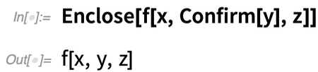 But now let’s put $Failed in place of y. $Failed is something that Confirm by default considers to be a problem. So when it sees $Failed, it stops, exiting to the Enclose—which in turn yields a Failure object:
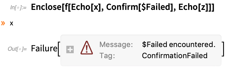
 If we put in some echoes, we’ll see that x is successfully reached, but z is not; as soon as the Confirm fails, it stops everything:
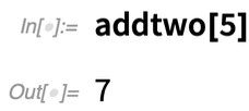
 A very common thing is to want to use Confirm/Enclose when you define a function:
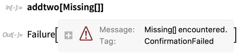
 But if we instead use Missing[]—which Confirm by default considers to be a problem—we get back a Failure object:
 We could achieve the same thing with If, Return, etc. But even in this very simple case, it wouldn’t look as nice.
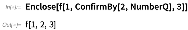
Confirm has a certain default set of things that it considers “wrong” ($Failed, Failure[...], Missing[...] are examples). But there are related functions that allow you to specify particular tests. For example, ConfirmBy applies a function to test if an expression should be confirmed.
Here, ConfirmBy confirms that 2 is a number:
We could achieve the same thing with If, Return, etc. But even in this very simple case, it wouldn’t look as nice.
Confirm has a certain default set of things that it considers “wrong” ($Failed, Failure[...], Missing[...] are examples). But there are related functions that allow you to specify particular tests. For example, ConfirmBy applies a function to test if an expression should be confirmed.
Here, ConfirmBy confirms that 2 is a number:
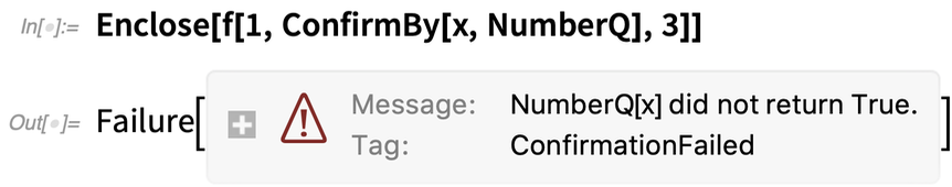
 But x is not considered so by NumberQ:
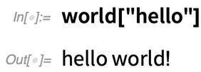
 OK, so let’s put these pieces together. Let’s define a function that’s supposed to operate on strings:
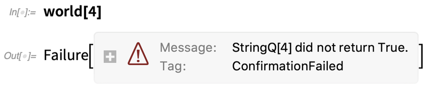
 But if we give it a number instead, the ConfirmBy fails:
 But here’s where really nice things start to happen. Let’s say we want to map world over a list, always confirming that it gets a good result. Here everything is OK:
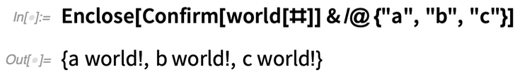 But now something has gone wrong:
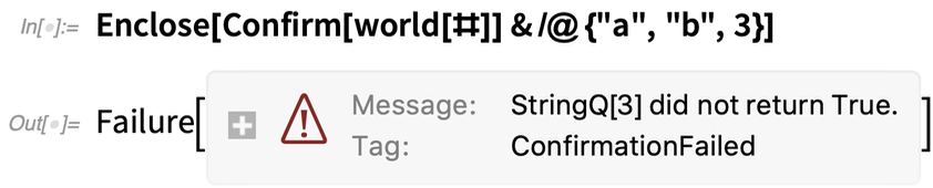 The ConfirmBy inside the definition of world failed, causing its enclosing Enclose to produce a Failure object. Then this Failure object caused the Confirm inside the Map to fail, and the enclosing Enclose gave a Failure object for the whole thing. Once again, we could have achieved the same thing with If, Throw, Catch, etc. But Confirm/Enclose do it more robustly, and more elegantly.
These are all very small examples. But where Confirm/Enclose really show their value is in large programs, and in providing a clear, high-level framework for handling errors and exceptions, and defining their scope.
In addition to Confirm and ConfirmBy, there’s also ConfirmMatch, which confirms that an expression matches a specified pattern. Then there’s ConfirmQuiet, which confirms that the evaluation of an expression doesn’t generate any messages (or, at least, none that you told it to test for). There’s also ConfirmAssert, which simply takes an “assertion” (like p>0) and confirms that it’s true.
When a confirmation fails, the program always exits to the nearest enclosing Enclose, delivering to the Enclose a Failure object with information about the failure that occurred. When you set up the Enclose, you can tell it how to handle failure objects it receives—either just returning them (perhaps to enclosing Confirm’s and Enclose’s), or applying functions to their contents.
Confirm and Enclose are an elegant mechanism for handling errors, that are easy and clean to insert into programs. But—needless to say—there are definitely some tricky issues around them. Let me mention just one. The question is: which Confirm’s does a given Enclose really enclose? If you’ve written a piece of code that explicitly contains Enclose and Confirm, it’s pretty obvious. But what if there’s a Confirm that’s somehow generated—perhaps dynamically—deep inside some stack of functions? It’s similar to the situation with named variables. Module just looks for the variables directly (“lexically”) inside its body. Block looks for variables (“dynamically”) wherever they may occur. Well, Enclose by default works like Module, “lexically” looking for Confirm’s to enclose. But if you include tags in Confirm and Enclose, you can set them up to “find each other” even if they’re not explicitly “visible” in the same piece of code.
The ConfirmBy inside the definition of world failed, causing its enclosing Enclose to produce a Failure object. Then this Failure object caused the Confirm inside the Map to fail, and the enclosing Enclose gave a Failure object for the whole thing. Once again, we could have achieved the same thing with If, Throw, Catch, etc. But Confirm/Enclose do it more robustly, and more elegantly.
These are all very small examples. But where Confirm/Enclose really show their value is in large programs, and in providing a clear, high-level framework for handling errors and exceptions, and defining their scope.
In addition to Confirm and ConfirmBy, there’s also ConfirmMatch, which confirms that an expression matches a specified pattern. Then there’s ConfirmQuiet, which confirms that the evaluation of an expression doesn’t generate any messages (or, at least, none that you told it to test for). There’s also ConfirmAssert, which simply takes an “assertion” (like p>0) and confirms that it’s true.
When a confirmation fails, the program always exits to the nearest enclosing Enclose, delivering to the Enclose a Failure object with information about the failure that occurred. When you set up the Enclose, you can tell it how to handle failure objects it receives—either just returning them (perhaps to enclosing Confirm’s and Enclose’s), or applying functions to their contents.
Confirm and Enclose are an elegant mechanism for handling errors, that are easy and clean to insert into programs. But—needless to say—there are definitely some tricky issues around them. Let me mention just one. The question is: which Confirm’s does a given Enclose really enclose? If you’ve written a piece of code that explicitly contains Enclose and Confirm, it’s pretty obvious. But what if there’s a Confirm that’s somehow generated—perhaps dynamically—deep inside some stack of functions? It’s similar to the situation with named variables. Module just looks for the variables directly (“lexically”) inside its body. Block looks for variables (“dynamically”) wherever they may occur. Well, Enclose by default works like Module, “lexically” looking for Confirm’s to enclose. But if you include tags in Confirm and Enclose, you can set them up to “find each other” even if they’re not explicitly “visible” in the same piece of code.Function Robustification
Confirm/Enclose provide a good high-level way to handle the “flow” of things going wrong inside a program or a function. But what if there’s something wrong right at the get-go? In our built-in Wolfram Language functions, there’s a standard set of checks we apply. Are there the correct number of arguments? If there are options, are they allowed options, and are they in the correct place? In Version 12.2 we’ve added two functions that can perform these standard checks for functions you write. This says that f should have two arguments, which here it doesn’t: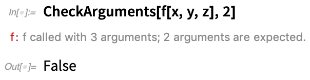 Here’s a way to make CheckArguments part of the basic definition of a function:
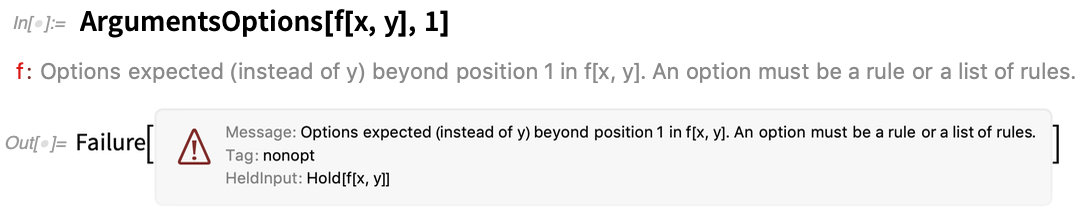
 ArgumentsOptions is another new function in Version 12.2—that separates “positional arguments” from options in a function. Set up options for a function:
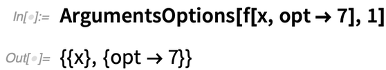 If it doesn’t find exactly one positional argument, it generates a message:
Cleaning Up After Your Code
You run a piece of code and it does what it does—and typically you don’t want it to leave anything behind. Often you can use scoping constructs like Module, Block, BlockRandom, etc. to achieve this. But sometimes there’ll be something you set up that needs to be explicitly “cleaned up” when your code finishes. For example, you might create a file in your piece of code, and want the file removed when that particular piece of code finishes. In Version 12.2 there’s a convenient new function for managing things like this: WithCleanup. WithCleanup[expr, cleanup] evaluates expr, then cleanup—but returns the result from expr. Here’s a trivial example (which could really be achieved better with Block). You’re assigning a value to x, getting its square—then clearing x before returning the square: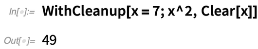 It’s already convenient just to have a construct that does cleanup while still returning the main expression you were evaluating. But an important detail of WithCleanup is that it also handles the situation where you abort the main evaluation you were doing. Normally, issuing an abort would cause everything to stop. But WithCleanup is set up to make sure that the cleanup happens even if there’s an abort. So if the cleanup involves, for example, deleting a file, the file gets deleted, even if the main operation is aborted.
WithCleanup also allows an initialization to be given. So here the initialization is done, as is the cleanup, but the main evaluation is aborted:
It’s already convenient just to have a construct that does cleanup while still returning the main expression you were evaluating. But an important detail of WithCleanup is that it also handles the situation where you abort the main evaluation you were doing. Normally, issuing an abort would cause everything to stop. But WithCleanup is set up to make sure that the cleanup happens even if there’s an abort. So if the cleanup involves, for example, deleting a file, the file gets deleted, even if the main operation is aborted.
WithCleanup also allows an initialization to be given. So here the initialization is done, as is the cleanup, but the main evaluation is aborted:
 By the way, WithCleanup can also be used with Confirm/Enclose to ensure that even if a confirmation fails, certain cleanup will be done.
Dates—with 37 New Calendars
It’s December 16, 2020, today—at least according to the standard Gregorian calendar that’s usually used in the US. But there are many other calendar systems in use for various purposes around the world, and even more that have been used at one time or another historically. In earlier versions of Wolfram Language we supported a few common calendar systems. But in Version 12.2 we’ve added very broad support for calendar systems—altogether 41 of them. One can think of calendar systems as being a bit like projections in geodesy or coordinate systems in geometry. You have a certain time: now you have to know how it is represented in whatever system you’re using. And much like GeoProjectionData, there’s now CalendarData which can give you a list of available calendar systems: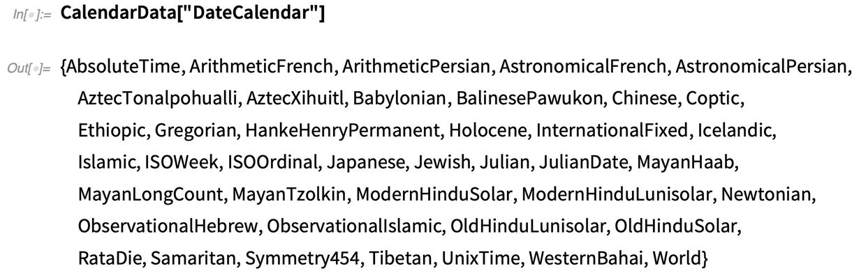 So here’s the representation of “now” converted to different calendars:
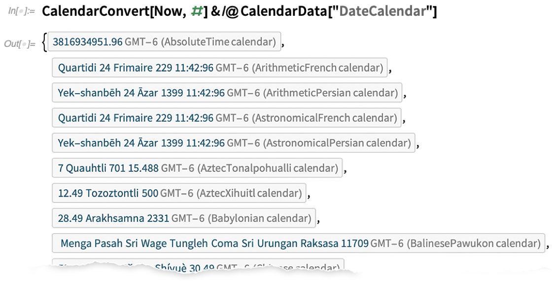 There are many subtleties here. Some calendars are purely “arithmetic”; others rely on astronomical computations. And then there’s the matter of “leap variants”. With the Gregorian calendar, we’re used to just adding a February 29. But the Chinese calendar, for example, can add whole “leap months” within a year (so that, for example, there can be two “fourth months”). In the Wolfram Language, we now have a symbolic representation for such things, using LeapVariant:
 One reason to deal with different calendar systems is that they’re used to determine holidays and festivals in different cultures. (Another reason, particularly relevant to someone like me who studies history quite a bit is in the conversion of historical dates: Newton’s birthday was originally recorded as December 25, 1642, but converting it to a Gregorian date it’s January 4, 1643.)
Given a calendar, something one often wants to do is to select dates that satisfy a particular criterion. And in Version 12.2 we’ve introduced the function DateSelect to do this. So, for example, we can select dates within a particular interval that satisfy the criterion that they are Wednesdays:
One reason to deal with different calendar systems is that they’re used to determine holidays and festivals in different cultures. (Another reason, particularly relevant to someone like me who studies history quite a bit is in the conversion of historical dates: Newton’s birthday was originally recorded as December 25, 1642, but converting it to a Gregorian date it’s January 4, 1643.)
Given a calendar, something one often wants to do is to select dates that satisfy a particular criterion. And in Version 12.2 we’ve introduced the function DateSelect to do this. So, for example, we can select dates within a particular interval that satisfy the criterion that they are Wednesdays:
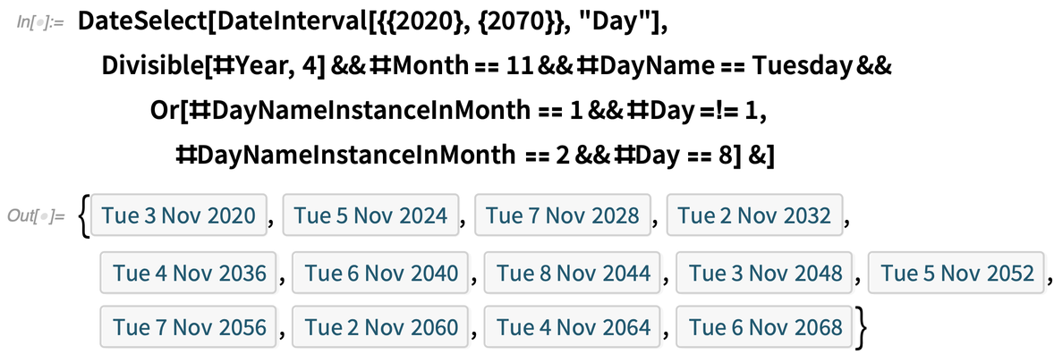
 As a more complicated example, we can convert the current algorithm for selecting dates of US presidential elections to computable form, and then use it to determine dates for the next 50 years:
New in Geo
By now, the Wolfram Language has strong capabilities in geo computation and geo visualization. But we’re continuing to expand our geo functionality. In Version 12.2 an important addition is spatial statistics (mentioned above)—which is fully integrated with geo. But there are also a couple of new geo primitives. One is GeoBoundary, which computes boundaries of things: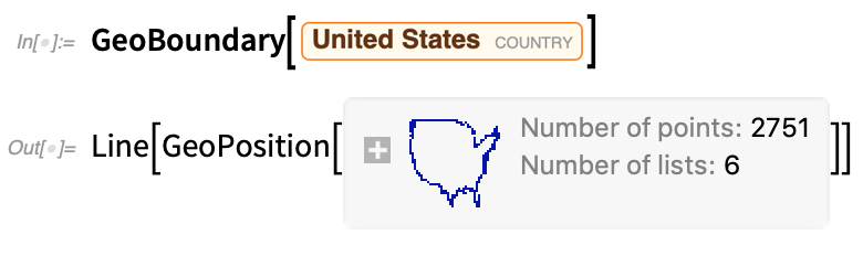
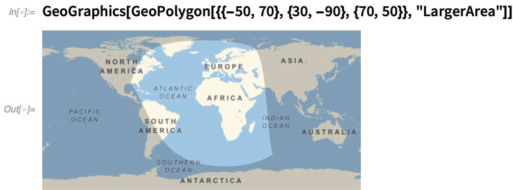
 There’s also GeoPolygon, which is a full geo generalization of ordinary polygons. One of the tricky issues GeoPolygon has to handle is what counts as the “interior” of a polygon on the Earth. Here it’s picking the larger area (i.e. the one that wraps around the globe):
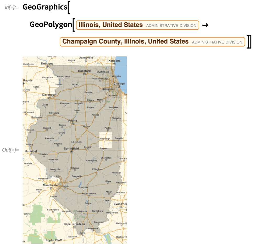
 GeoPolygon can also—like Polygon—handle holes, or in fact arbitrary levels of nesting:
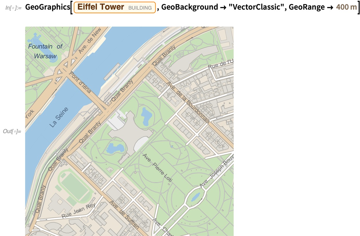
 But the biggest “coming attraction” of geo is completely new rendering of geo graphics and maps. It’s still preliminary (and unfinished) in Version 12.2, but there’s at least experimental support for vector-based map rendering. The most obvious payoff from this is maps that look much crisper and sharper at all scales. But another payoff is our ability to introduce new styling for maps, and in Version 12.2 we’re including eight new map styles.
Here’s our “old-style”map:
But the biggest “coming attraction” of geo is completely new rendering of geo graphics and maps. It’s still preliminary (and unfinished) in Version 12.2, but there’s at least experimental support for vector-based map rendering. The most obvious payoff from this is maps that look much crisper and sharper at all scales. But another payoff is our ability to introduce new styling for maps, and in Version 12.2 we’re including eight new map styles.
Here’s our “old-style”map:
 Here’s the new, vector version of this “classic” style:
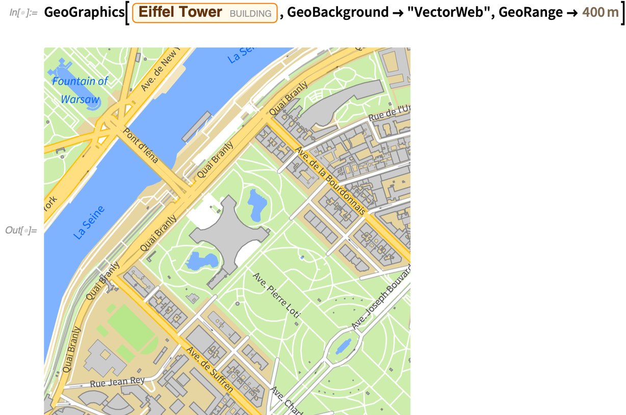
 Here’s a new (vector) style, intended for the web:
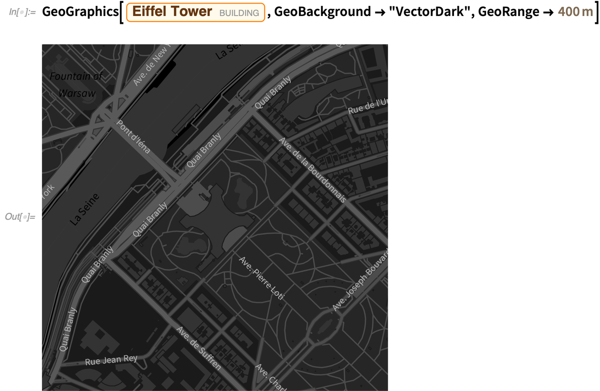
 And here’s a “dark” style, suitable for having information overlaid on it:
Importing PDF
Want to analyze a document that’s in PDF? We’ve been able to extract basic content from PDF files for well over a decade. But PDF is a highly complex (and evolving) format, and many documents “in the wild” have complicated structure. In Version 12.2, however, we’ve dramatically expanded our PDF import capabilities, so that it becomes realistic to, for example, take a random paper from arXiv, and import it: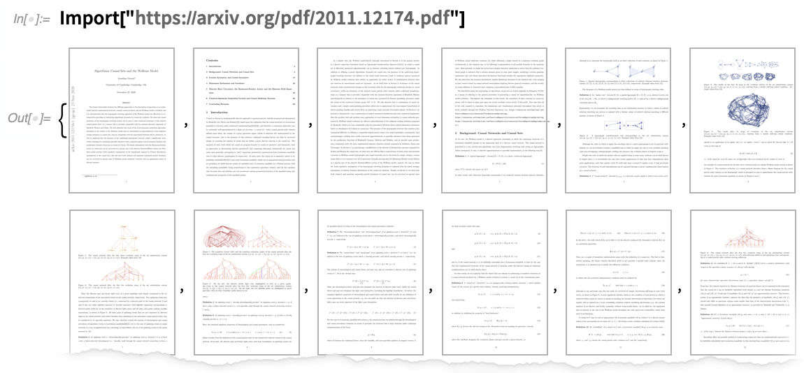 By default, what you’ll get is a high-resolution image for each page (in this particular case, all 100 pages).
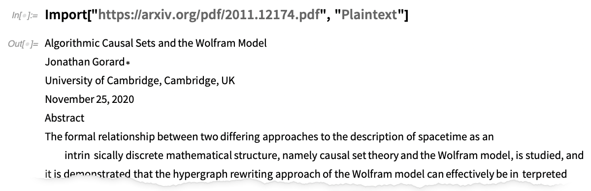
If you want the text, you can import that with “Plaintext”:
By default, what you’ll get is a high-resolution image for each page (in this particular case, all 100 pages).
If you want the text, you can import that with “Plaintext”:
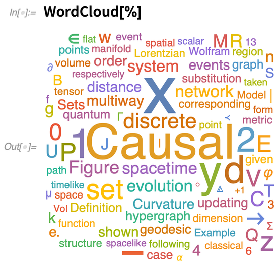
 Now you can immediately make a word cloud of the words in the paper:
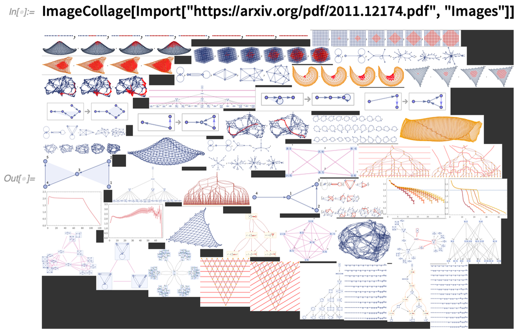
 This picks out all the images from the paper, and makes a collage of them:
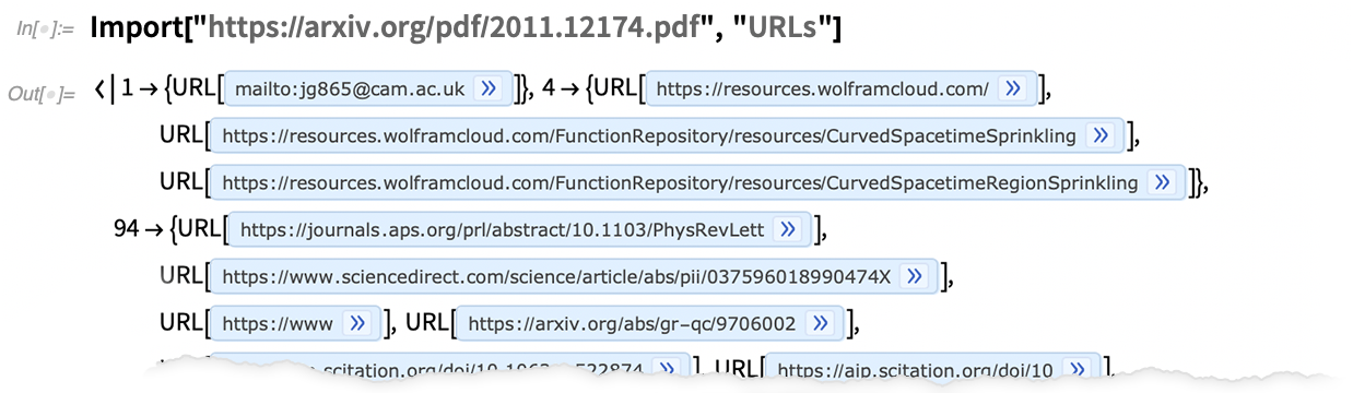
 You can get the URLs from each page:
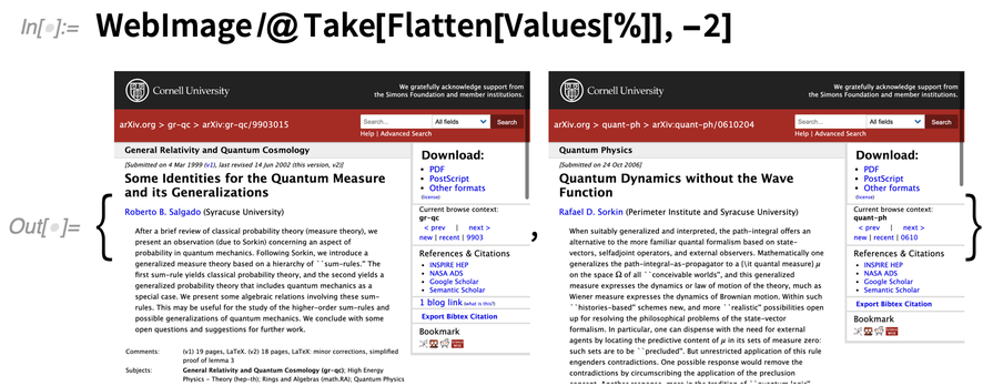
 Now pick off the last two, and get images of those webpages:
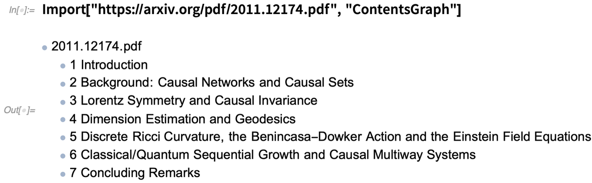
 Depending on how they’re produced, PDFs can have all sorts of structure. “ContentsGraph” gives a graph representing the overall structure detected for a document:
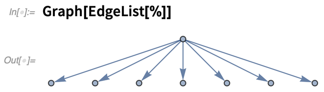
 And, yes, it really is a graph:
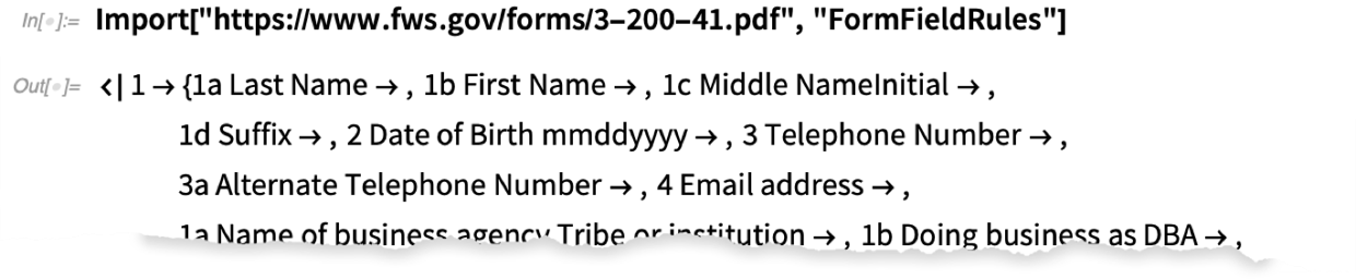
 For PDFs that are fillable forms, there’s more structure to import. Here I grabbed a random unfilled government form from the web. Import gives an association whose keys are the names of the fields—and if the form had been filled in, it would have given their values too, so you could immediately do analysis on them:
The Latest in Industrial-Strength Convex Optimization
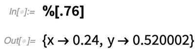
tarting in Version 12.0, we’ve been adding state-of-the-art capabilities for solving large-scale optimization problems. In Version 12.2 we’ve continued to round out these capabilities. One new thing is the superfunction ConvexOptimization, which automatically handles the full spectrum of linear, linear-fractional, quadratic, semidefinite and conic optimization—giving both optimal solutions and their dual properties. In 12.1 we added support for integer variables (i.e. combinatorial optimization); in 12.2 we’re also adding support for complex variables. But the biggest new things for optimization in 12.2 are the introduction of robust optimization and of parametric optimization. Robust optimization lets you find an optimum that’s valid across a whole range of values of some of the variables. Parametric optimization lets you get a parametric function that gives the optimum for any possible value of particular parameters. So for example this finds the optimum for x, y for any (positive) value of α: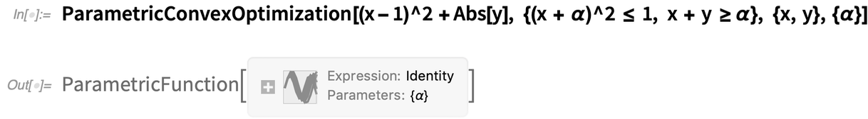 Now evaluate the parametric function for a particular α:
 As with everything in the Wolfram Language, we’ve put a lot of effort into making sure that convex optimization integrates seamlessly into the rest of the system—so you can set up models symbolically, and flow their results into other functions. We’ve also included some very powerful convex optimization solvers. But particularly if you’re doing mixed (i.e. real+integer) optimization, or you’re dealing with really huge (e.g. 10 million variables) problems, we’re also giving access to other, external solvers. So, for example, you can set up your problem using Wolfram Language as your “algebraic modeling language”, then (assuming you have the appropriate external licenses) just by setting Method to, say, “Gurobi” or “Mosek” you can immediately run your problem with an external solver. (And, by the way, we now have an open framework for adding more solvers.)
Supporting Combinators and Other Formal Building Blocks
One can say that the whole idea of symbolic expressions (and their transformations) on which we rely so much in the Wolfram Language originated with combinators—which just celebrated their centenary on December 7, 2020. The version of symbolic expressions that we have in Wolfram Language is in many ways vastly more advanced and usable than raw combinators. But in Version 12.2—partly by way of celebrating combinators—we wanted to add a framework for raw combinators. So now for example we have CombinatorS, CombinatorK, etc., rendered appropriately: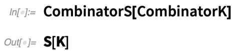 But how should we represent the application of one combinator to another? Today we write something like:
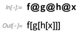 But in the early days of mathematical logic there was a different convention—that involved left-associative application, in which one expected “combinator style” to generate “functions” not “values” from applying functions to things. So in Version 12.2 we’re introducing a new “application operator” Application, displayed as (and entered as \[Application] or ap ):
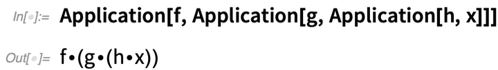
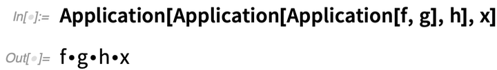 And, by the way, I fully expect Application—as a new, basic “constructor”—to have a variety of uses (not to mention “applications”) in setting up general structures in the Wolfram Language.
The rules for combinators are trivial to specify using pattern transformations in the Wolfram Language:
And, by the way, I fully expect Application—as a new, basic “constructor”—to have a variety of uses (not to mention “applications”) in setting up general structures in the Wolfram Language.
The rules for combinators are trivial to specify using pattern transformations in the Wolfram Language:
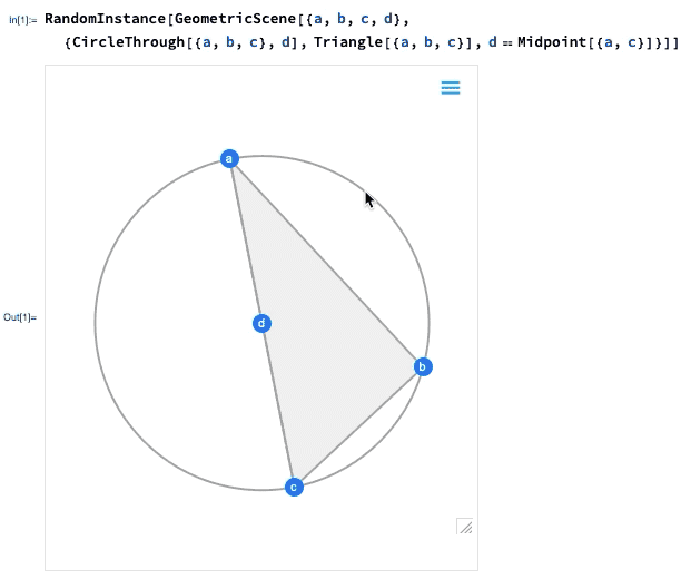
Euclidean Geometry Goes Interactive
One of the major advances in Version 12.0 was the introduction of a symbolic representation for Euclidean geometry: you specify a symbolic GeometricScene, giving a variety of objects and constraints, and the Wolfram Language can “solve” it, and draw a diagram of a random instance that satisfies the constraints. In Version 12.2 we’ve made this interactive, so you can move the points in the diagram around, and everything will (if possible) interactively be rearranged so as to maintain the constraints.
Here’s a random instance of a simple geometric scene:
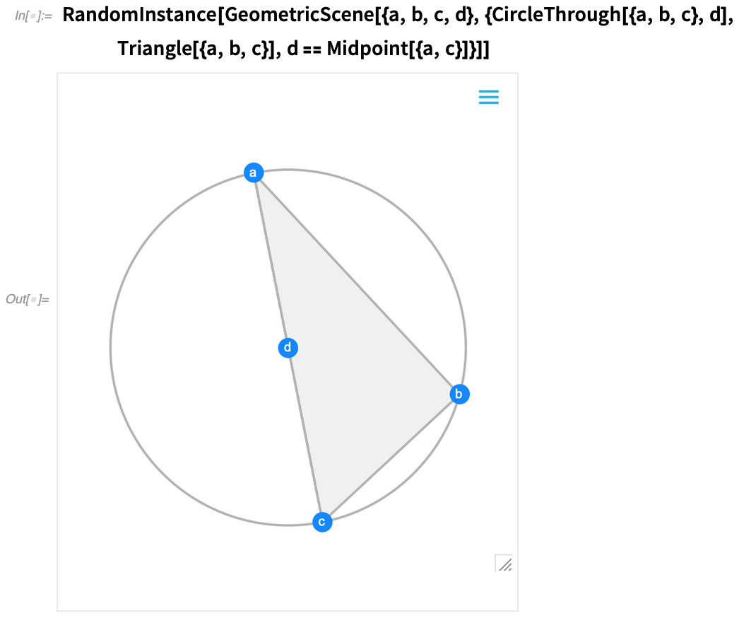
If you move one of the points, the other points will interactively be rearranged so as to maintain the constraints defined in the symbolic representation of the geometric scene:
What’s really going on inside here? Basically, the geometry is getting converted to algebra. And if you want, you can get the algebraic formulation:
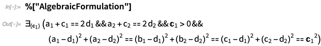
And, needless to say, you can manipulate this using the many powerful algebraic computation capabilities of the Wolfram Language. In addition to interactivity, another major new feature in 12.2 is the ability to handle not just complete geometric scenes, but also geometric constructions that involve building up a scene in multiple steps. Here’s an example—that happens to be taken directly from Euclid:
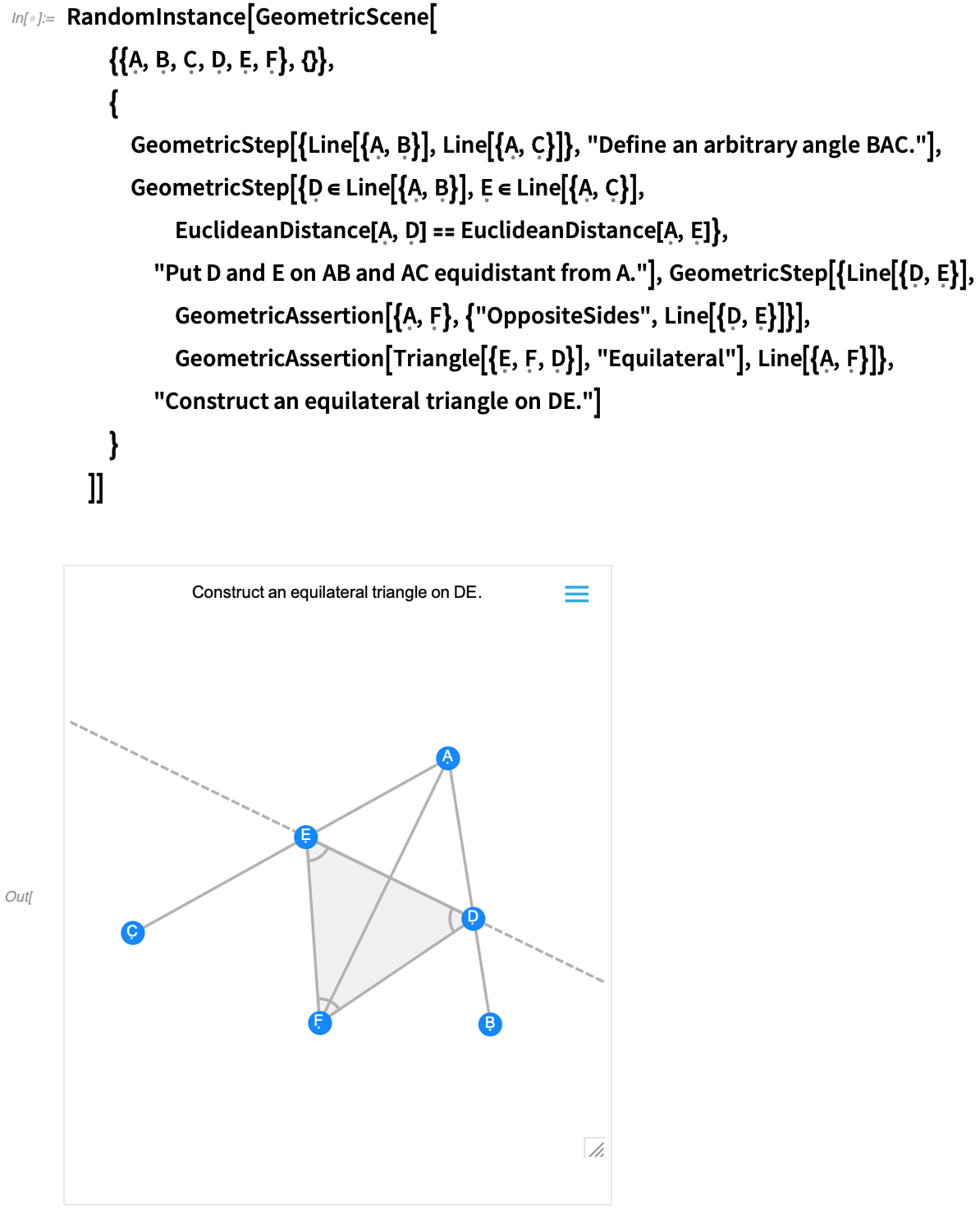
The first image you get is basically the result of the construction. And—like all other geometric scenes—it’s now interactive. But if you mouse over it, you’ll get controls that allow you to move to earlier steps:
Move a point at an earlier step, and you’ll see what consequences that has for later steps in the construction. Euclid’s geometry is the very first axiomatic system for mathematics that we know about. So—2000+ years later—it’s exciting that we can finally make it computable. (And, yes, it will eventually connect up with AxiomaticTheory, FindEquationalProof, etc.)
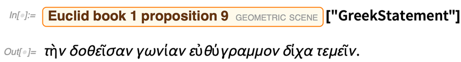
But in recognition of the significance of Euclid’s original formulation of geometry, we’ve added computable versions of his propositions (as well as a bunch of other “famous geometric theorems”). The example above turns out to be proposition 9 in Euclid’s book 1. And now, for example, we can get his original statement of it in Greek:
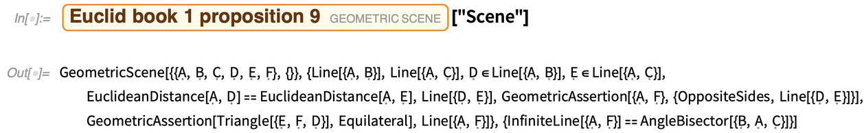
And here it is in modern Wolfram Language—in a form that can be understood by both computers and humans:
Yet More Kinds of Knowledge for the Knowledgebase
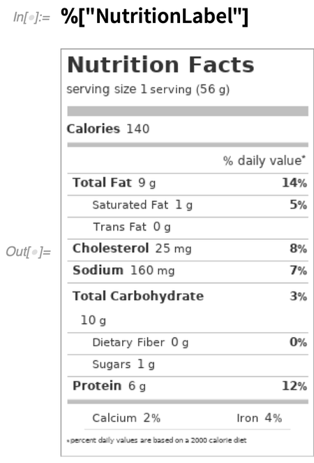
An important part of the story of Wolfram Language as a full-scale computational language is its access to our vast knowledgebase of data about the world. The knowledgebase is continually being updated and expanded, and indeed in the time since Version 12.1 essentially all domains have had data (and often a substantial amount) updated, or entities added or modified. But as examples of what’s been done, let me mention a few additions. One area that’s received a lot of attention is food. By now we have data about more than half a million foods (by comparison, a typical large grocery store stocks perhaps 30,000 types of items). Pick a random food: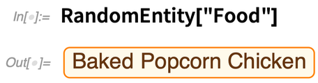 Now generate a nutrition label:
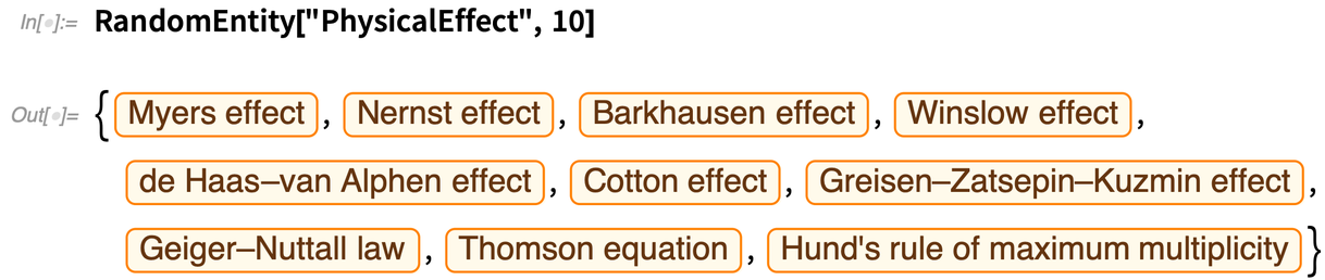
 As another example, a new type of entity that’s been added is physical effects. Here are some random ones:
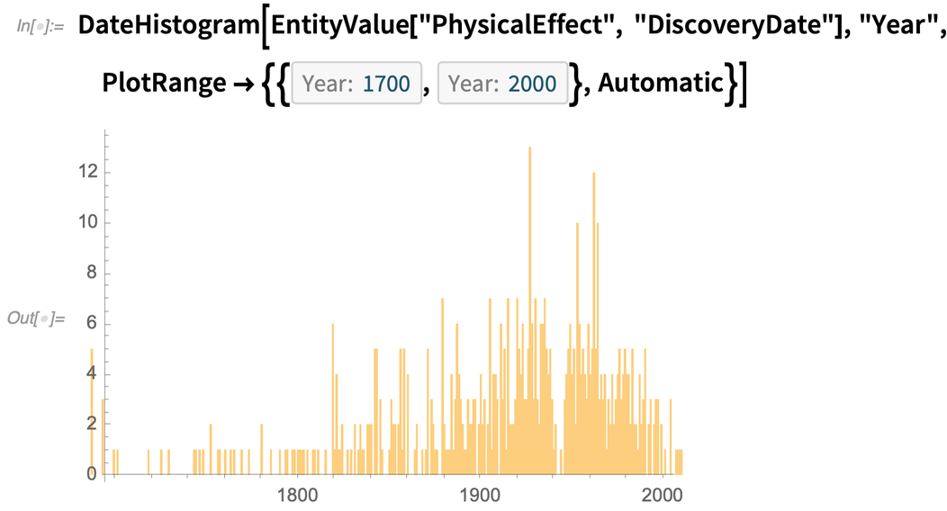
 And as an example of something that can be done with all the data in this domain, here’s a histogram of the dates when these effects were discovered:
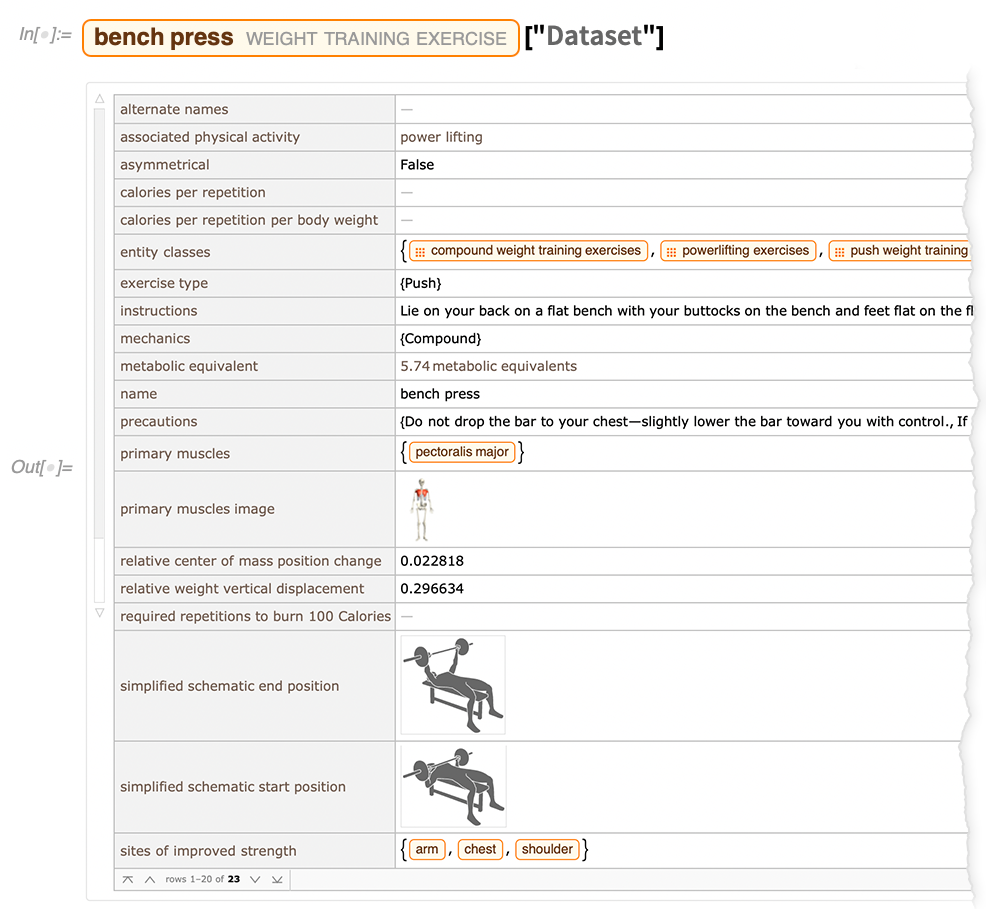
 As another sample of what we’ve been up to, there’s also now what one might (tongue-in-cheek) call a “heavy-lifting” domain—weight-training exercises:
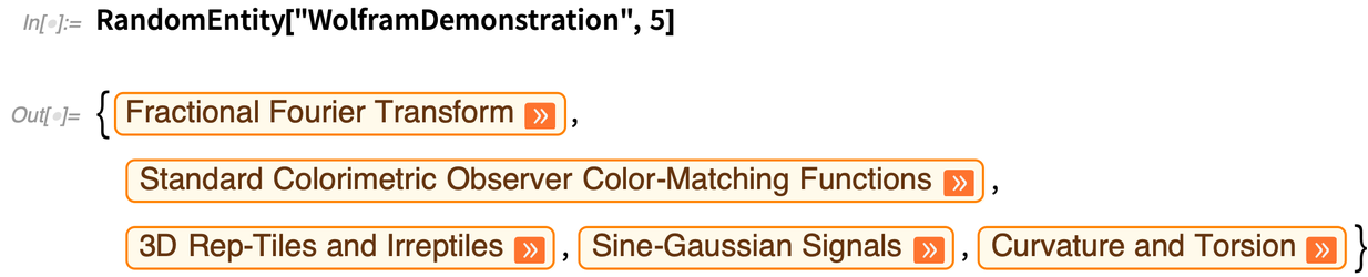
 An important feature of the Wolfram Knowledgebase is that it contains symbolic objects, which can represent not only “plain data”—like numbers or strings—but full computational content. And as an example of this, Version 12.2 allows one to access the Wolfram Demonstrations Project—with all its active Wolfram Language code and notebooks—directly in the knowledgebase. Here are some random Demonstrations:
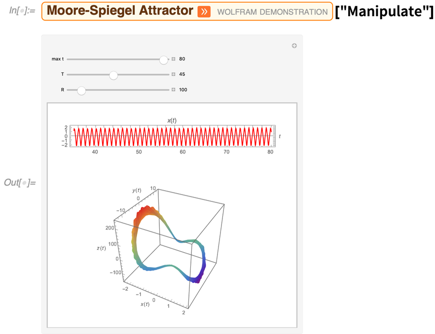
 The values of properties can be dynamic interactive objects:
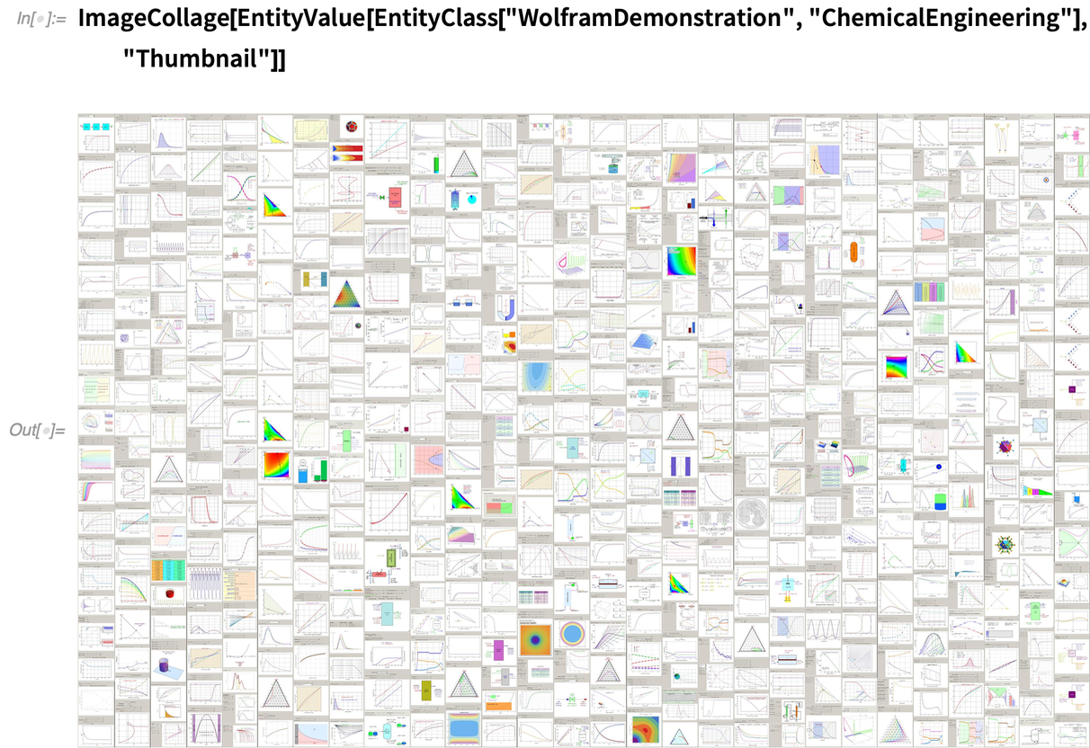
 And because everything is computable, one can for example immediately make an image collage of all Demonstrations on a particular topic:
The Continuing Story of Machine Learning
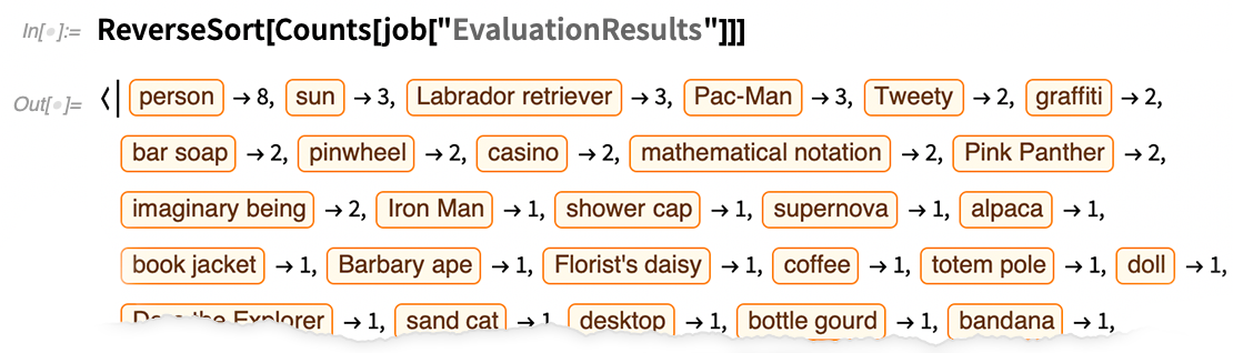
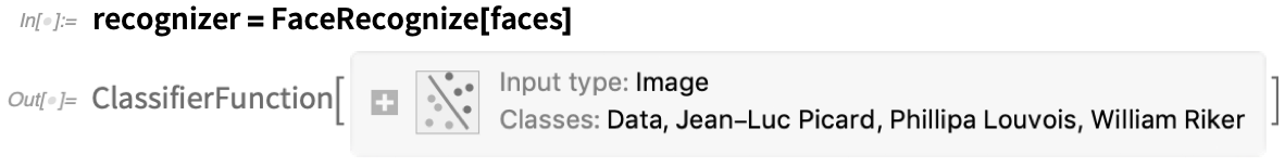
It’s been nearly 7 years since we first introduced Classify and Predict, and began the process of fully integrating neural networks into the Wolfram Language. There’ve been two major directions: the first is to develop “superfunctions”, like Classify and Predict, that—as automatically as possible—perform machine-learning-based operations. The second direction is to provide a powerful symbolic framework to take advantage of the latest advances with neural nets (notably through the Wolfram Neural Net Repository) and to allow flexible continued development and experimentation. Version 12.2 has progress in both these areas. An example of a new superfunction is FaceRecognize. Give it a small number of tagged examples of faces, and it will try to identify them in images, videos, etc. Let’s get some training data from web searches (and, yes, it’s somewhat noisy): Now create a face recognizer with this training data:
 Now we can use this to find out who’s on screen in each frame of a video:
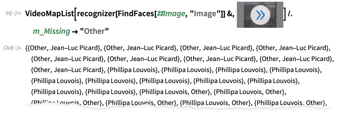 Now plot the results:
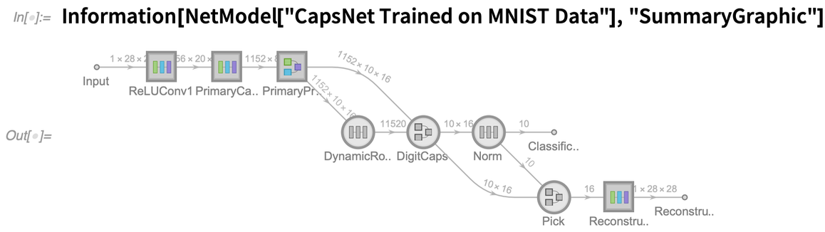
 In the Wolfram Neural Net Repository there’s a regular stream of new networks being added. Since Version 12.1 about 20 new kinds of networks have been added—including many new transformer nets, as well as EfficientNet and for example feature extractors like BioBERT and SciBERT specifically trained on text from scientific papers.
In each case, the networks are immediately accessible—and usable—through NetModel. Something that’s updated in Version 12.2 is the visual display of networks:
In the Wolfram Neural Net Repository there’s a regular stream of new networks being added. Since Version 12.1 about 20 new kinds of networks have been added—including many new transformer nets, as well as EfficientNet and for example feature extractors like BioBERT and SciBERT specifically trained on text from scientific papers.
In each case, the networks are immediately accessible—and usable—through NetModel. Something that’s updated in Version 12.2 is the visual display of networks:
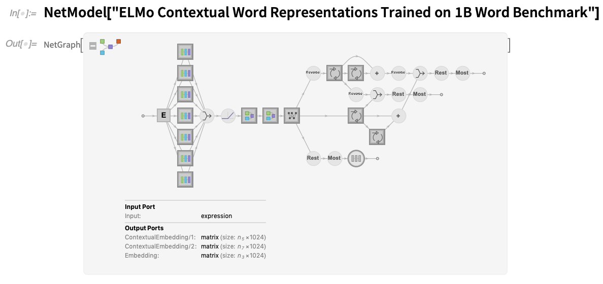 There are lots of new icons, but there’s also now a clear convention that circles represent fixed elements of a net, while squares represent trainable ones. In addition, when there’s a thick border in an icon, it means there’s an additional network inside, that you can see by clicking. Whether it’s a network that comes from NetModel or your construct yourself (or a combination of those two), it’s often convenient to extract the “summary graphic” for the network, for example so you can put it in documentation or a publication. Information provides several levels of summary graphics:
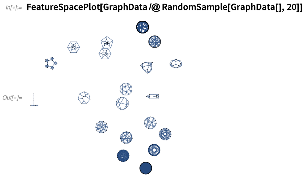
 There are several important additions to our core neural net framework that broaden the range of neural net functionality we can access. The first is that in Version 12.2 we have native encoders for graphs and for time series. So, here, for example, we’re making a feature space plot of 20 random named graphs:
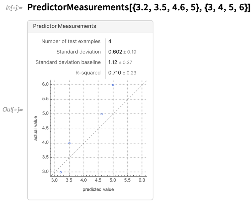
 Another enhancement to the framework has to do with diagnostics for models. We introduced PredictorMeasurements and ClassifierMeasurements many years ago to provide a symbolic representation for the performance of models. In Version 12.2—in response to many requests—we’ve made it possible to feed final predictions, rather than a model, to create a PredictorMeasurements object, and we’ve streamlined the appearance and operation of PredictorMeasurements objects:
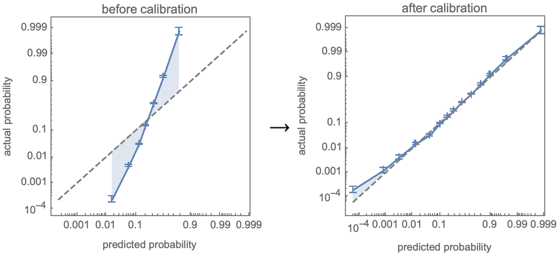
 An important new feature of ClassifierMeasurements is the ability to compute a calibration curve that compares the actual probabilities observed from sampling a test set with the predictions from the classifier. But what’s even more important is that Classify automatically calibrates its probabilities, in effect trying to “sculpt” the calibration curve:
 Version 12.2 also has the beginning of a major update to the way neural networks can be constructed. The fundamental setup has always been to put together a certain collection of layers that expose what amount to array indices that are connected by explicit edges in a graph. Version 12.2 now introduces FunctionLayer, which allows you to give something much closer to ordinary Wolfram Language code. As an example, here’s a particular function layer:
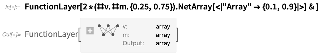 And here’s the representation of this function layer as an explicit NetGraph:
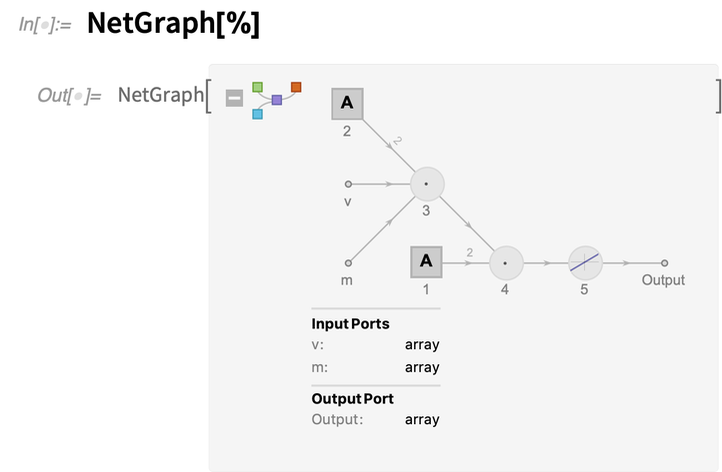 v and m are named “input ports”. The NetArray—indicated by the square icons in the net graph—is a learnable array, here containing just two elements.
There are cases where it’s easier to use the “block-based” (or “graphical”) programming approach of just connecting together layers (and we’ve worked hard to ensure that the connections can be made as automatically as possible). But there are also cases where it’s easier to use the “functional” programming approach of FunctionLayer. For now, FunctionLayer supports only a subset of the constructs available in the Wolfram Language—though this already includes many standard array and functional programming operations, and more will be added in the future.
An important feature of FunctionLayer is that the neural net it produces will be as efficient as any other neural net, and can run on GPUs etc. But what can you do about Wolfram Language constructs that are not yet natively supported by FunctionLayer? In Version 12.2 we’re adding another new experimental function—CompiledLayer—that extends the range of Wolfram Language code that can be handled efficiently.
It’s perhaps worth explaining a bit about what’s happening inside. Our main neural net framework is essentially a symbolic layer that organizes things for optimized low-level implementation, currently using MXNet. FunctionLayer is effectively translating certain Wolfram Language constructs directly to MXNet. CompiledLayer is translating Wolfram Language to LLVM and then to machine code, and inserting this into the execution process within MXNet. CompiledLayer makes use of the new Wolfram Language compiler, and its extensive type inference and type declaration mechanisms.
OK, so let’s say one’s built a magnificent neural net in our Wolfram Language framework. Everything is set up so that the network can immediately be used in a whole range of Wolfram Language superfunctions (Classify, FeatureSpacePlot, AnomalyDetection, FindClusters, …). But what if one wants to use the network “standalone” in an external environment? In Version 12.2 we’re introducing the capability to export essentially any network in the recently developed ONNX standard representation.
And once one has a network in ONNX form, one can use the whole ecosystem of external tools to deploy it in a wide variety of environments. A notable example—that’s now a fairly streamlined process—is to take a full Wolfram Language–created neural net and run it in CoreML on an iPhone, so that it can for example directly be included in a mobile app.
v and m are named “input ports”. The NetArray—indicated by the square icons in the net graph—is a learnable array, here containing just two elements.
There are cases where it’s easier to use the “block-based” (or “graphical”) programming approach of just connecting together layers (and we’ve worked hard to ensure that the connections can be made as automatically as possible). But there are also cases where it’s easier to use the “functional” programming approach of FunctionLayer. For now, FunctionLayer supports only a subset of the constructs available in the Wolfram Language—though this already includes many standard array and functional programming operations, and more will be added in the future.
An important feature of FunctionLayer is that the neural net it produces will be as efficient as any other neural net, and can run on GPUs etc. But what can you do about Wolfram Language constructs that are not yet natively supported by FunctionLayer? In Version 12.2 we’re adding another new experimental function—CompiledLayer—that extends the range of Wolfram Language code that can be handled efficiently.
It’s perhaps worth explaining a bit about what’s happening inside. Our main neural net framework is essentially a symbolic layer that organizes things for optimized low-level implementation, currently using MXNet. FunctionLayer is effectively translating certain Wolfram Language constructs directly to MXNet. CompiledLayer is translating Wolfram Language to LLVM and then to machine code, and inserting this into the execution process within MXNet. CompiledLayer makes use of the new Wolfram Language compiler, and its extensive type inference and type declaration mechanisms.
OK, so let’s say one’s built a magnificent neural net in our Wolfram Language framework. Everything is set up so that the network can immediately be used in a whole range of Wolfram Language superfunctions (Classify, FeatureSpacePlot, AnomalyDetection, FindClusters, …). But what if one wants to use the network “standalone” in an external environment? In Version 12.2 we’re introducing the capability to export essentially any network in the recently developed ONNX standard representation.
And once one has a network in ONNX form, one can use the whole ecosystem of external tools to deploy it in a wide variety of environments. A notable example—that’s now a fairly streamlined process—is to take a full Wolfram Language–created neural net and run it in CoreML on an iPhone, so that it can for example directly be included in a mobile app.Form Notebooks
What’s the best way to collect structured material? If you just want to get a few items, an ordinary form created with FormFunction (and for example deployed in the cloud) can work well. But what if you’re trying to collect longer, richer material? For example, let’s say you’re creating a quiz where you want students to enter a whole sequence of complex responses. Or let’s say you’re creating a template for people to fill in documentation for something. What you need in these cases is a new concept that we’re introducing in Version 12.2: form notebooks. A form notebook is basically a notebook that is set up to be used as a complex “form”, where the inputs in the form can be all the kinds of things that you’re used to having in a notebook. The basic workflow for form notebooks is the following. First you author a form notebook, defining the various “form elements” (or areas) that you want the user of the form notebook to fill in. As part of the authoring process, you define what you want to have happen to the material the user of the form notebook enters when they use the form notebook (e.g. put the material in a Wolfram Data Drop databin, send the material to a cloud API, send the material as a symbolic expression by email, etc.). After you’ve authored the form notebook, you then generate an active version that can be sent to whoever will be using the form notebook. Once someone has filled in their material in their copy of the deployed form notebook, they press a button, typically “Submit”, and their material is then sent as a structured symbolic expression to whatever destination the author of the form notebook specified. It’s perhaps worth mentioning how form notebooks relate to something that sounds similar: template notebooks. In a sense, a template notebook is doing the reverse of a form notebook. A form notebook is about having a user enter material that will then be processed. A template notebook, on the other hand, is about having the computer generate material which will then be used to populate a notebook whose structure is defined by the template notebook. OK, so how do you get started with form notebooks? Just go to File > New > Programmatic Notebook > Form Notebook Authoring: This is just a notebook, where you can enter whatever content you want—say an explanation of what you want people to do when they “fill out” the form notebook. But then there are special cells or sequences of cells in the form notebook that we call “form elements” and “editable notebook areas”. These are what the user of the form notebook “fills out” to enter their “responses”, and the material they provide is what gets sent when they press the “Submit” button (or whatever final action has been defined).
In the authoring notebook, the toolbar gives you a menu of possible form elements that you can insert:
This is just a notebook, where you can enter whatever content you want—say an explanation of what you want people to do when they “fill out” the form notebook. But then there are special cells or sequences of cells in the form notebook that we call “form elements” and “editable notebook areas”. These are what the user of the form notebook “fills out” to enter their “responses”, and the material they provide is what gets sent when they press the “Submit” button (or whatever final action has been defined).
In the authoring notebook, the toolbar gives you a menu of possible form elements that you can insert:
 Let’s pick “Input Field” as an example:
 What does all this mean? Basically a form element is represented by a very flexible symbolic Wolfram Language expression, and this is giving you a way to specify the expression you want. You can give a label and a hint to put in the input field. But it’s with the Interpreter that you start to see the power of Wolfram Language. Because the Interpreter is what takes whatever the user of the form notebooks enters in this input field, and interprets it as a computable object. The default is just to treat it as a string. But it could for example be a “Country” or a “MathExpression”. And with these choices, the material will automatically be interpreted as a country, math expression, etc., with the user typically being prompted if their input can’t be interpreted as specified.
There are lots of options about the details of how even an input field can work. Some of them are provided in the Add Action menu:
What does all this mean? Basically a form element is represented by a very flexible symbolic Wolfram Language expression, and this is giving you a way to specify the expression you want. You can give a label and a hint to put in the input field. But it’s with the Interpreter that you start to see the power of Wolfram Language. Because the Interpreter is what takes whatever the user of the form notebooks enters in this input field, and interprets it as a computable object. The default is just to treat it as a string. But it could for example be a “Country” or a “MathExpression”. And with these choices, the material will automatically be interpreted as a country, math expression, etc., with the user typically being prompted if their input can’t be interpreted as specified.
There are lots of options about the details of how even an input field can work. Some of them are provided in the Add Action menu:
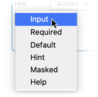 But so what actually “is” this form element? Press the CODE tab on the left to see:
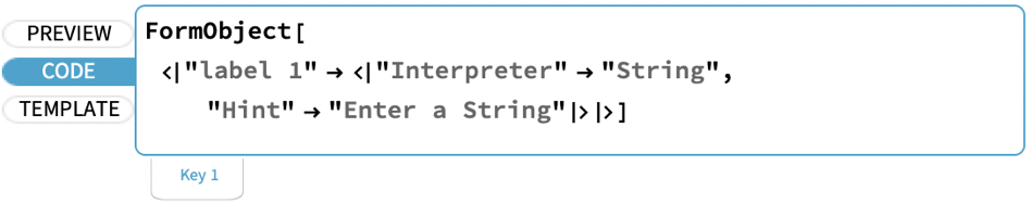 What would a user of the form notebook see here? Press the PREVIEW tab to find out:
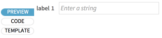 Beyond input fields, there are lots of other possible form elements. There are things like checkboxes, radio buttons and sliders. And in general it’s possible to use any of the rich symbolic user interface constructs that exist in the Wolfram Language.
Once you’ve finishing authoring, you press Generate to generate a form notebook that is ready to be provided to users to be filled in. The Settings define things like how the “submit” action should be specified, and what should be done when the form notebook is submitted:
Beyond input fields, there are lots of other possible form elements. There are things like checkboxes, radio buttons and sliders. And in general it’s possible to use any of the rich symbolic user interface constructs that exist in the Wolfram Language.
Once you’ve finishing authoring, you press Generate to generate a form notebook that is ready to be provided to users to be filled in. The Settings define things like how the “submit” action should be specified, and what should be done when the form notebook is submitted:
 So what is the “result” of a submitted form notebook? Basically it’s an association that says what was filled into each area of the form notebook. (The areas are identified by keys in the association that were specified when the areas were first defined in the authoring notebook.)
Let’s see how this works in a simple case. Here’s the authoring notebook for a form notebook:
So what is the “result” of a submitted form notebook? Basically it’s an association that says what was filled into each area of the form notebook. (The areas are identified by keys in the association that were specified when the areas were first defined in the authoring notebook.)
Let’s see how this works in a simple case. Here’s the authoring notebook for a form notebook:
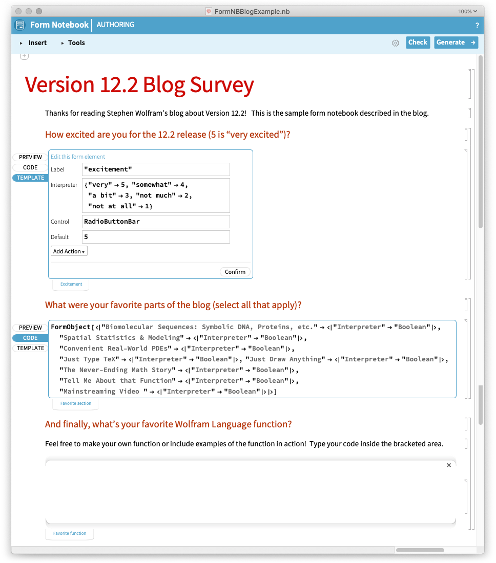 Here’s the generated form notebook, ready to be filled in:
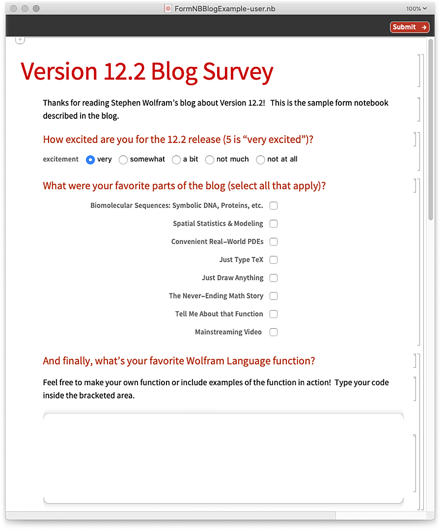 Here’s a sample of how the form notebook might be filled in:
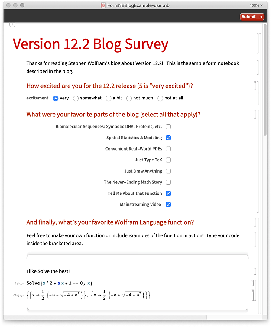 And this is what “comes back” when Submit is pressed:
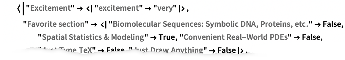 For testing, you can just have this association placed interactively in a notebook. But in practice it’s more common to send the association to a databin, store it in a cloud object, or generally put it in a more “centralized” location.
Notice that at the end of this example we have an editable notebook area—where you can enter free-form notebook content (with cells, headings, code, output, etc.) that will all be captured when the form notebook is submitted. Form notebooks are very powerful idea, and you’ll see them used all over the place. As a first example, the various submission notebooks for the Wolfram Function Repository, Wolfram Demonstrations Project, etc. are becoming form notebooks. We’re also expecting a lot of use of form notebooks in educational settings. And as part of that, we’re building a system that leverages Wolfram Language for assessing responses in form notebooks (and elsewhere).
You can see the beginnings of this in Version 12.2 with the experimental function AssessmentFunction—which can be hooked into form notebooks somewhat like Interpreter. But even without the full capabilities planned for AssessmentFunction there’s still an incredible amount that can be done—in educational settings and otherwise—using form notebooks.
It’s worth understanding, by the way, that form notebooks are ultimately very simple to use in any particular case. Yes, they have a lot of depth that allows them to do a very wide range of things. And they’re basically only possible because of the whole symbolic structure of the Wolfram Language, and the fact that Wolfram Notebooks are ultimately represented as symbolic expressions. But when it comes to using them for a particular purpose they’re very streamlined and straightforward, and it’s completely realistic to create a useful form notebook in just a few minutes.
For testing, you can just have this association placed interactively in a notebook. But in practice it’s more common to send the association to a databin, store it in a cloud object, or generally put it in a more “centralized” location.
Notice that at the end of this example we have an editable notebook area—where you can enter free-form notebook content (with cells, headings, code, output, etc.) that will all be captured when the form notebook is submitted. Form notebooks are very powerful idea, and you’ll see them used all over the place. As a first example, the various submission notebooks for the Wolfram Function Repository, Wolfram Demonstrations Project, etc. are becoming form notebooks. We’re also expecting a lot of use of form notebooks in educational settings. And as part of that, we’re building a system that leverages Wolfram Language for assessing responses in form notebooks (and elsewhere).
You can see the beginnings of this in Version 12.2 with the experimental function AssessmentFunction—which can be hooked into form notebooks somewhat like Interpreter. But even without the full capabilities planned for AssessmentFunction there’s still an incredible amount that can be done—in educational settings and otherwise—using form notebooks.
It’s worth understanding, by the way, that form notebooks are ultimately very simple to use in any particular case. Yes, they have a lot of depth that allows them to do a very wide range of things. And they’re basically only possible because of the whole symbolic structure of the Wolfram Language, and the fact that Wolfram Notebooks are ultimately represented as symbolic expressions. But when it comes to using them for a particular purpose they’re very streamlined and straightforward, and it’s completely realistic to create a useful form notebook in just a few minutes.Yet More Notebookery
We invented notebooks—with all their basic features of hierarchical cells, etc.—back in 1987. But for a third of a century, we’ve been progressively polishing and streamlining how they work. And in Version 12.2 there are all sorts of useful and convenient new notebook features. Click to Copy It’s a very simple feature, but it’s very useful. You see something in a notebook, and all you really want to be able to do with it is copy it (or perhaps copy something related to it). Well, then just use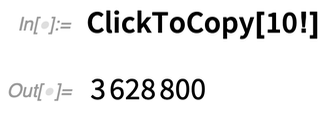 If you want to click-to-copy something unevaluated, use Defer:
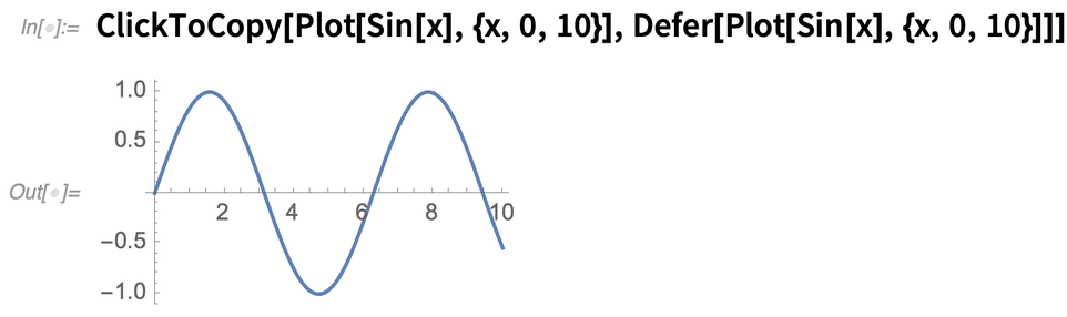 Streamlined Hyperlinking (and Hyperlink Editing)
++h has inserted a hyperlink in a Wolfram Notebook since 1996. But in Version 12.2 there are two important new things with hyperlinks. First, automatic hyperlinking that handles a wide range of different situations. And second, a modernized and streamlined mechanism for hyperlink creation and editing.
Streamlined Hyperlinking (and Hyperlink Editing)
++h has inserted a hyperlink in a Wolfram Notebook since 1996. But in Version 12.2 there are two important new things with hyperlinks. First, automatic hyperlinking that handles a wide range of different situations. And second, a modernized and streamlined mechanism for hyperlink creation and editing.
 Attached Cells
In Version 12.2 we’re exposing something that we’ve had internally for a while: the ability to attach a floating fully functional cell to any given cell (or box, or whole notebook). Accessing this feature needs symbolic notebook programming, but it lets you do very powerful things—particularly in introducing contextual and “just-in-time” interfaces. Here’s an example that puts a dynamic counter that counts in primes on right-bottom part of the cell bracket:
Attached Cells
In Version 12.2 we’re exposing something that we’ve had internally for a while: the ability to attach a floating fully functional cell to any given cell (or box, or whole notebook). Accessing this feature needs symbolic notebook programming, but it lets you do very powerful things—particularly in introducing contextual and “just-in-time” interfaces. Here’s an example that puts a dynamic counter that counts in primes on right-bottom part of the cell bracket:
 Template Box InfrastructureSometimes it’s useful for what you see not to be what you have. For example, you might want to display something in a notebook as J0(x) but have it really be BesselJ[0, x]. For many years, we’ve had Interpretation as a way to set this up for specific expressions. But we’ve also had a more general mechanism—TemplateBox—that lets you take expressions, and separately specify how they should be displayed, and interpreted.
In Version 12.2 we’ve further generalized—and streamlined—TemplateBox, allowing it to incorporate arbitrary user interface elements, as well as allowing it to specify things like copy behavior. Our new TEX input mechanism, for example, is basically just an application of the new TemplateBox.
In this case, "TeXAssistantTemplate" refers to a piece of functionality defined in the notebook stylesheet—whose parameters are specified by the association given in the TemplateBox:
Template Box InfrastructureSometimes it’s useful for what you see not to be what you have. For example, you might want to display something in a notebook as J0(x) but have it really be BesselJ[0, x]. For many years, we’ve had Interpretation as a way to set this up for specific expressions. But we’ve also had a more general mechanism—TemplateBox—that lets you take expressions, and separately specify how they should be displayed, and interpreted.
In Version 12.2 we’ve further generalized—and streamlined—TemplateBox, allowing it to incorporate arbitrary user interface elements, as well as allowing it to specify things like copy behavior. Our new TEX input mechanism, for example, is basically just an application of the new TemplateBox.
In this case, "TeXAssistantTemplate" refers to a piece of functionality defined in the notebook stylesheet—whose parameters are specified by the association given in the TemplateBox:
The Desktop Interface to the Cloud
An important feature of Wolfram Notebooks is that they’re set up to operate both on the desktop and in the cloud. And even between versions of Wolfram Language there’s lots of continued enhancement in the way notebooks work in the cloud. But in Version 12.2 there’s been some particular streamlining of the interface for notebooks between desktop and cloud. A particularly nice mechanism already available for a couple of years in any desktop notebook is the File > Publish to Cloud… menu item, which allows you to take the notebook and immediately make it available as a published cloud notebook that can be accessed by anyone with a web browser. In Version 12.2 we’ve streamlined the process of notebook publishing. When I’m giving a presentation I’ll usually be creating a desktop notebook as I go (or perhaps using one that already exists). And at the end of the presentation, it’s become my practice to publish it to the cloud, so anyone in the audience can interact with it. But how can I give everyone the URL for the notebook? In a virtual setting, you can just use chat. But in an actual physical presentation, that’s not an option. And in Version 12.2 we’ve provided a convenient alternative: the result of Publish to Cloud includes a QR code that people can capture with their phones, then immediately go to the URL and interact with the notebook on their phones. There’s one other notable new item visible in the result of Publish to Cloud: “Direct JavaScript Embedding”. This is a link to the Wolfram Notebook Embedder which allows cloud notebooks to be directly embedded through JavaScript onto webpages.
It’s always easy to use an iframe to embed one webpage on another. But iframes have many limitations, such as requiring their size to be defined in advance. The Wolfram Notebook Embedder allows full-function fluid embedding of cloud notebooks—as well as scriptable control of the notebooks from other elements of a webpage. And since the Wolfram Notebook Embedder is set up to use the oEmbed embedding standard, it can immediately be used in basically all standard web content management systems.
We’ve talked about sending notebooks from the desktop to the cloud. But another thing that’s new in Version 12.2 is faster and easier browsing of your cloud file system from the desktop—as accessed from File > Open from Cloud… and File > Save to Cloud…
There’s one other notable new item visible in the result of Publish to Cloud: “Direct JavaScript Embedding”. This is a link to the Wolfram Notebook Embedder which allows cloud notebooks to be directly embedded through JavaScript onto webpages.
It’s always easy to use an iframe to embed one webpage on another. But iframes have many limitations, such as requiring their size to be defined in advance. The Wolfram Notebook Embedder allows full-function fluid embedding of cloud notebooks—as well as scriptable control of the notebooks from other elements of a webpage. And since the Wolfram Notebook Embedder is set up to use the oEmbed embedding standard, it can immediately be used in basically all standard web content management systems.
We’ve talked about sending notebooks from the desktop to the cloud. But another thing that’s new in Version 12.2 is faster and easier browsing of your cloud file system from the desktop—as accessed from File > Open from Cloud… and File > Save to Cloud…
Cryptography & Security
One of the things we want to do with Wolfram Language is to make it as easy as possible to connect with pretty much any external system. And in modern times an important part of that is being able to conveniently handle cryptographic protocols. And ever since we started introducing cryptography directly into the Wolfram Language five years ago, I’ve been surprised at just how much the symbolic character of the Wolfram Language has allowed us to clarify and streamline things to do with cryptography. A particularly dramatic example of this has been how we’ve been able to integrate blockchains into Wolfram Language (and Version 12.2 adds bloxberg with several more on the way). And in successive versions we’re handling different applications of cryptography. In Version 12.2 a major emphasis is symbolic capabilities for key management. Version 12.1 already introduced SystemCredential for dealing with local “keychain” key management (supporting, for example, “remember me” in authentication dialogs). In 12.2 we’re also dealing with PEM files. If we import a PEM file containing a private key we get a nice, symbolic representation of the private key: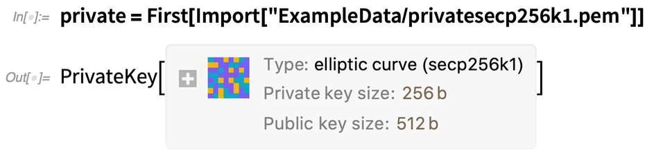 Now we can derive a public key:
 If we generate a digital signature for a message using the private key
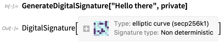 then this verifies the signature using the public key we’ve derived:
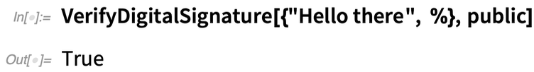 An important part of modern security infrastructure is the concept of a security certificate—a digital construct that allows a third party to attest to the authenticity of a particular public key. In Version 12.2 we now have a symbolic representation for security certificates—providing what’s needed for programs to establish secure communication channels with outside entities in the same kind of way that https does:
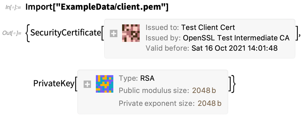
Just Type SQL
In Version 12.0 we introduced powerful functionality for querying relational databases symbolically within the Wolfram Language. Here’s how we connect to a database: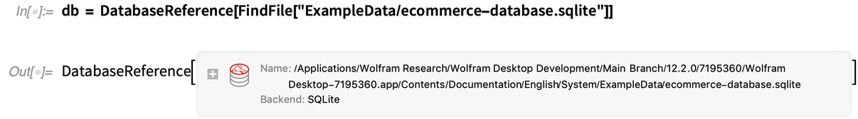 Here’s how we connect the database so that its tables can be treated just like entity types from the built-in Wolfram Knowledgebase:
 Now we can for example ask for a list of entities of a given type:
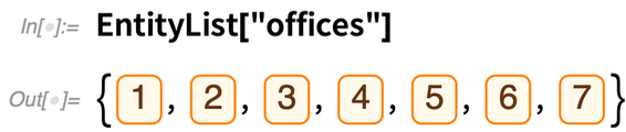 What’s new in 12.2 is that we can conveniently go “under” this layer, to directly execute SQL queries against the underlying database, getting the complete database table as a Dataset expression:
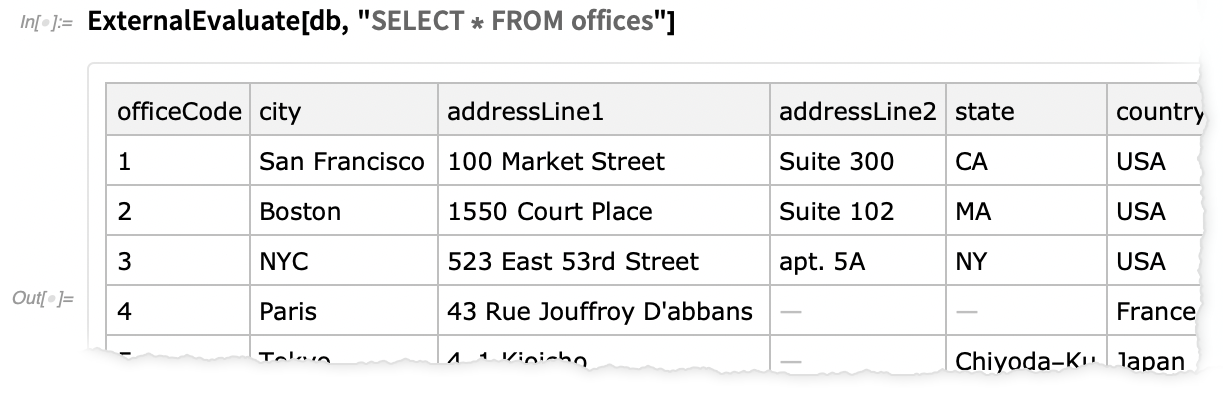 These queries can not only read from the database, but also write to it. And to make things even more convenient, we can effectively treat SQL just like any other “external language” in a notebook.
First we have to register our database, to say what we want our SQL to be run against:
These queries can not only read from the database, but also write to it. And to make things even more convenient, we can effectively treat SQL just like any other “external language” in a notebook.
First we have to register our database, to say what we want our SQL to be run against:
 And now we can just type SQL as input—and get back Wolfram Language output, directly in the notebook:

Microcontroller Support Goes 32 Bit
You’ve developed a control system or signal processing in Wolfram Language. Now how do you deploy it to a piece of standalone electronics? In Version 12.0 we introduced the Microcontroller Kit for compiling from symbolic Wolfram Language structures directly to microcontroller code. We’ve had lots of feedback on this, asking us to expand the range of microcontrollers that we support. So in Version 12.2 I’m happy to say that we’re adding support for 36 new microcontrollers, particularly 32-bit ones: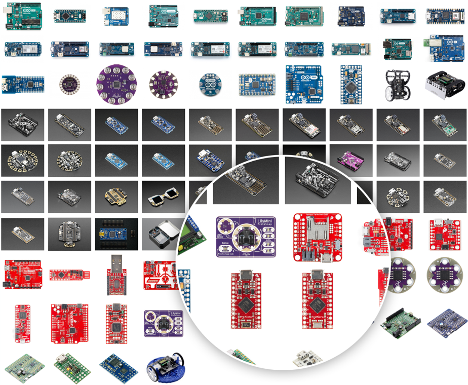 Here’s an example in which we deploy a symbolically defined digital filter to a particular kind of microcontroller, showing the simplified C source code generated for that particular microcontroller:
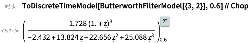
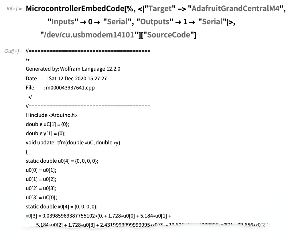
WSTPServer: A New Deployment of Wolfram Engine
Our long-term goal is to make the Wolfram Language and the computational intelligence it provides as ubiquitous as possible. And part of doing this is to set up the Wolfram Engine which implements the language so that it can be deployed in as broad a range of computational infrastructure settings as possible.
Wolfram Desktop—as well as classic Mathematica—primarily provide a notebook interface to the Wolfram Engine, running on a local desktop system. It’s also possible to run Wolfram Engine directly—as a command-line program (e.g. through WolframScript)—on a local computer system. And, of course, one can run the Wolfram Engine in the cloud, either through the full Wolfram Cloud (public or private), or through more lightweight cloud and server offerings (both existing and forthcoming).
But with Version 12.2 there’s a new deployment of the Wolfram Engine: WSTPServer. If you use Wolfram Engine in the cloud, you’re typically communicating with it through http or related protocols. But for more than thirty years, the Wolfram Language has had its own dedicated protocol for transferring symbolic expressions and everything around them. Originally we called it MathLink, but in more recent years, as it’s progressively been extended, we’ve called it WSTP: the Wolfram Symbolic Transfer Protocol. What WSTPServer does, as its name suggests, is to give you a lightweight server that delivers Wolfram Engines and lets you communicate with them directly in native WSTP.
Why is this important? Basically because it gives you a way to manage pools of persistent Wolfram Language sessions that can operate as services for other applications. For example, normally each time you call WolframScript you get a new, fresh Wolfram Engine. But by using wolframscript -wstpserver with a particular “WSTP profile name” you can keep getting the same Wolfram Engine every time you call WolframScript. You can do this directly on your local machine—or on remote machines.
And an important use of WSTPServer is to expose pools of Wolfram Engines that can be accessed through the new RemoteEvaluate function in Version 12.2. It’s also possible to use WSTPServer to expose Wolfram Engines for use by ParallelMap, etc. And finally, since WSTP has (for nearly 30 years!) been the way the notebook front end communicates with the Wolfram Engine kernel, it’s now possible to use WSTPServer to set up a centralized kernel pool to which you can connect the notebook front end, allowing you, for example, to keep running a particular session (or even a particular computation) in the kernel even as you switch to a different notebook front end, on a different computer.
RemoteEvaluate: Compute Someplace Else…
Along the lines of “use Wolfram Language everywhere” another new function in Version 12.2 is RemoteEvaluate. We’ve got CloudEvaluate which does a computation in the Wolfram Cloud, or an Enterprise Private Cloud. We’ve got ParallelEvaluate which does computations on a predefined collection of parallel subkernels. And in Version 12.2 we’ve got RemoteBatchSubmit which submits batch computations to cloud computation providers. RemoteEvaluate is a general, lightweight “evaluate now” function that lets you do a computation on any specified remote machine that has an accessible Wolfram Engine. You can connect to the remote machine using ssh or wstp (or http with a Wolfram Cloud endpoint).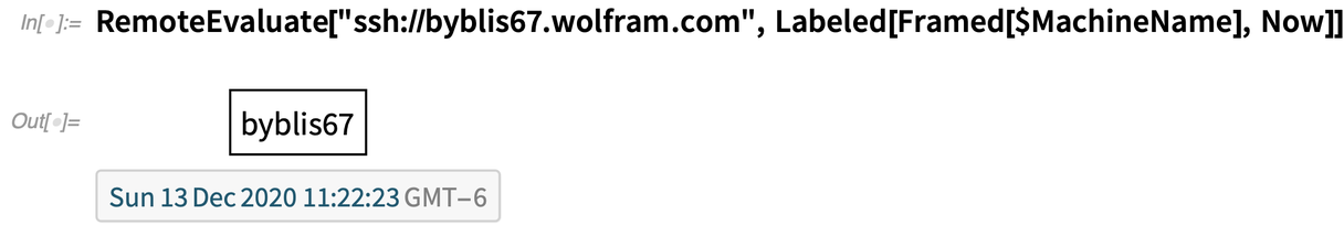 Sometimes you’ll want to use RemoteEvaluate to do things like system administration across a range of machines. Sometimes you might want to collect or send data to remote devices. For example, you might have a network of Raspberry Pi computers which all have Wolfram Engine—and then you can use RemoteEvaluate to do something like retrieve data from these machines. By the way, you can also use ParallelEvaluate from within RemoteEvaluate, so you’re having a remote machine be the master for a collection of parallel subkernels.
Sometimes you’ll want RemoteEvaluate to start a fresh instance of Wolfram Engine whenever you do an evaluation. But with WSTPServer you can also have it use a persistent Wolfram Language session. RemoteEvaluate and WSTPServer are the beginning of a general symbolic framework for representing running Wolfram Engine processes. Version 12.2 already has RemoteKernelObject and $DefaultRemoteKernel which provide symbolic ways to represent remote Wolfram Language instances.
Sometimes you’ll want to use RemoteEvaluate to do things like system administration across a range of machines. Sometimes you might want to collect or send data to remote devices. For example, you might have a network of Raspberry Pi computers which all have Wolfram Engine—and then you can use RemoteEvaluate to do something like retrieve data from these machines. By the way, you can also use ParallelEvaluate from within RemoteEvaluate, so you’re having a remote machine be the master for a collection of parallel subkernels.
Sometimes you’ll want RemoteEvaluate to start a fresh instance of Wolfram Engine whenever you do an evaluation. But with WSTPServer you can also have it use a persistent Wolfram Language session. RemoteEvaluate and WSTPServer are the beginning of a general symbolic framework for representing running Wolfram Engine processes. Version 12.2 already has RemoteKernelObject and $DefaultRemoteKernel which provide symbolic ways to represent remote Wolfram Language instances.And Yet More (AKA “None of the Above”)
I’ve at least touched on many of the bigger new features of Version 12.2. But there’s a lot more. Additional functions, enhancements, fixes and general rounding out and polishing.
Like in computational geometry, ConvexHullRegion now deals with regions, not just points. And there are functions like CollinearPoints and CoplanarPoints that test for collinearity and coplanarity, or give conditions for achieving them.
There are more import and export formats. Like there’s now support for the archive formats: “7z”, “ISO”, “RAR”, “ZSTD”. There’s also FileFormatQ and ByteArrayFormatQ for testing whether things correspond to particular formats.
In terms of core language, there are things like updates to the complicated-to-define ValueQ. There’s also RandomGeneratorState that gives a symbolic representation of random generator states.
In the desktop package (i.e. .wl file) editor, there’s a new (somewhat experimental) Format Cell button, that reformats code—with a control on how “airy” it should be (i.e. how dense it should be in newlines).
In Wolfram|Alpha-mode notebooks (as used by default in Wolfram|Alpha Notebook Edition) there are other new features, like function documentation targeted for particular function usage.
There’s also more in TableView, as well as a large suite of new paclet authoring tools that are included on an experimental basis.
To me it’s rather amazing how much we’ve been able to bring together in Version 12.2, and, as always, I’m excited that it’s now out and available to everyone to use….