Stata 18 provides the new estat gofplot command to produce goodness-of-fit (GOF) plots for survival models. You can use it after four survival models: right-censored Cox (stcox), interval-censored Cox (stintcox), right-censored parametric (streg), and interval-censored parametric (stintreg). Check model fit after stratified models or separately for each by-group.
GOF plots provide visual checks for how well the model fits the data. In survival analysis, these checks are based on so-called Cox–Snell residuals and the assumption that, if a model is correct, these residuals should have a standard exponential distribution. Visually, this assumption is assessed by plotting the residuals against their estimated cumulative hazard—the closer the plotted values are to the 45° line, the better the fit (Cox and Snell 1968).
Let’s see it work
GOF plots for right-censored data
We use the dataset on 103 patients admitted to the Stanford Heart Transplantation Program (Crowley and Hu 1977). The dataset includes the year the patient was accepted into the program (year), the patient’s age (age), whether the patient had other heart surgery previously (surgery), and whether the patient received a transplant (posttran). We wish to analyze time until death and check whether our model fits the data well. We fit a Cox model first by typing

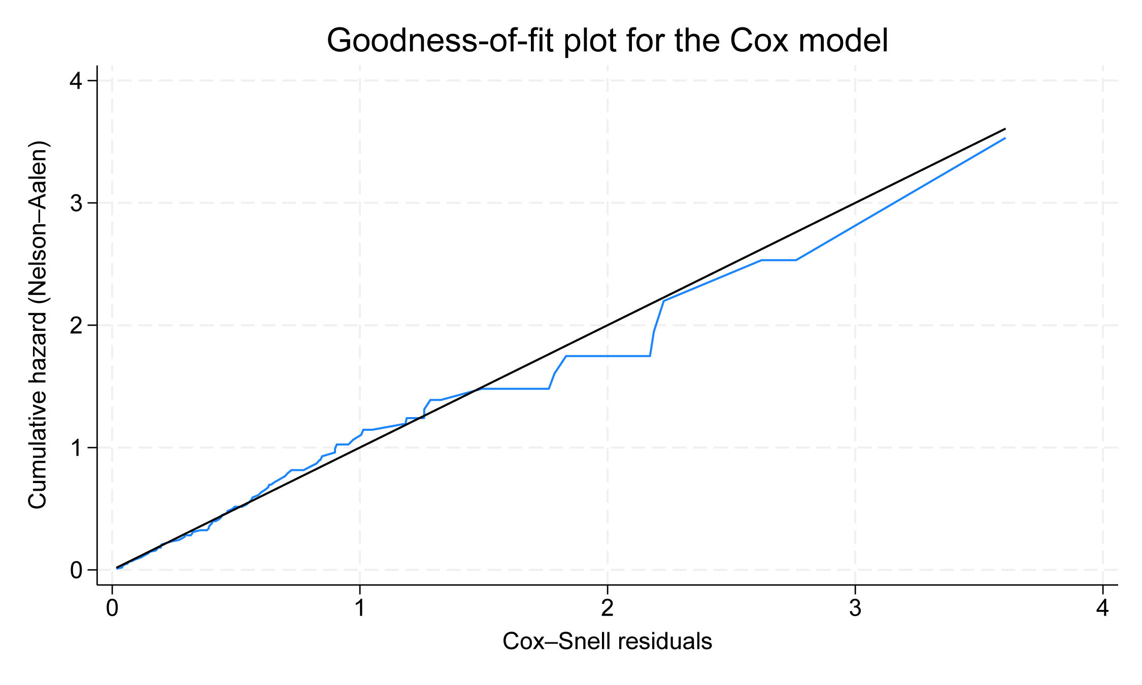
Comparing the blue line with the black reference line, we conclude that our Cox model fits the data well.
For right-censored data, instead of the default Nelson–Aalen estimator (Nelson 1972; Aalen 1978), we can use option km to use the alternative minus log of the Kaplan–Meier estimator (Kaplan and Meier 1958).
Let’s now fit a stratified Cox model, which assumes that the baseline hazard functions are different between patients from different groups (pgroup) but the coefficients are equal across those groups.
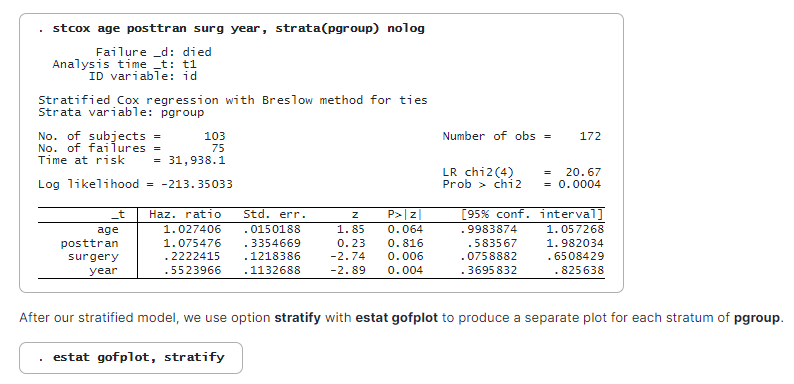
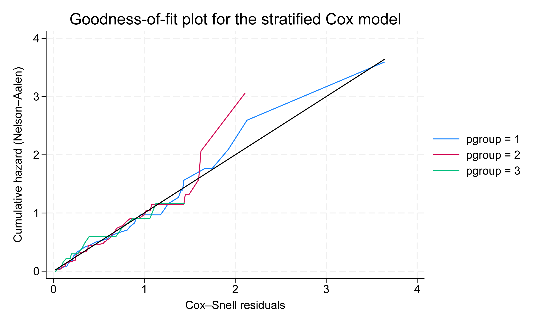
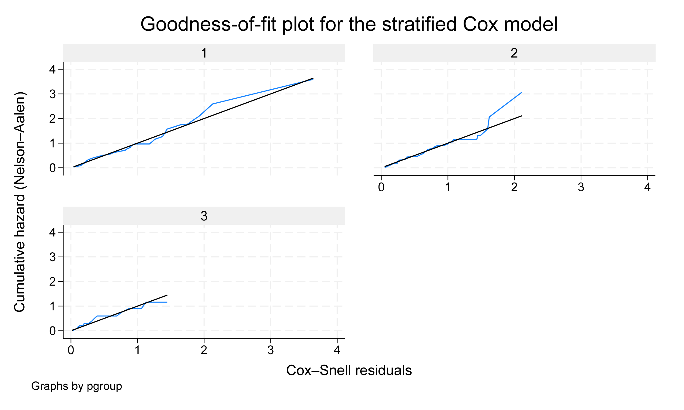
The model fits data well in all strata. The red line for pgroup = 2 deviates from the reference line toward the end. This is not uncommon to see in practice because fewer observations are available for estimation toward the end of the study.
To aid visual inspection of the plot, we can also add option separate to produce separate graphs for each stratum.
. estat gofplot, stratify separate
GOF plots for interval-censored data
We use the dataset of a study for early breast cancer patients (Finkelstein and Wolfe 1985) that compares the cosmetic effects of two cancer treatments (treat) on breast retraction. Because patients were observed at random follow-up times, the exact time of breast retraction was not observed and was known only to fall in the interval between visits (variables ltime and rtime). First, we fit an interval-censored Weibull model of time to breast retraction on treatment using stintreg:

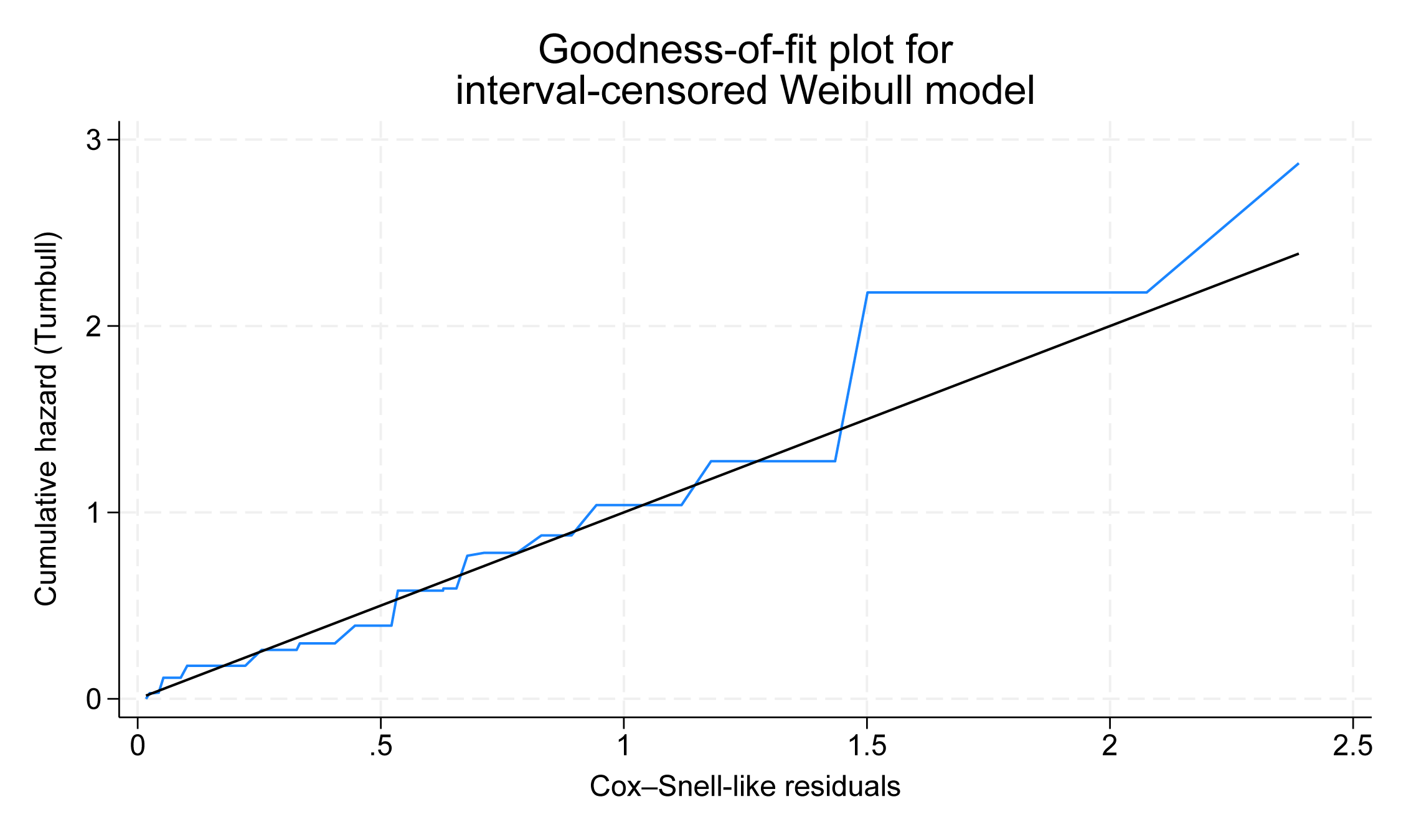
With interval-censored data, Cox–Snell-like residuals are defined and used for plotting (Farrington 2000). If a model fits the data well, these residuals should approximate the censored standard exponential distribution. Also, the nonparametric Turnbull estimator (Turnbull 1976) is used to estimate the cumulative hazard.
The jagged line stays close to the reference line in the above graph, which indicates that the Weibull model fits the data well.
Suppose that we now want to fit an exponential model and check its model fit. We type
. quietly stintreg i.treat, interval(ltime rtime) distribution(exponential)
. estat gofplot
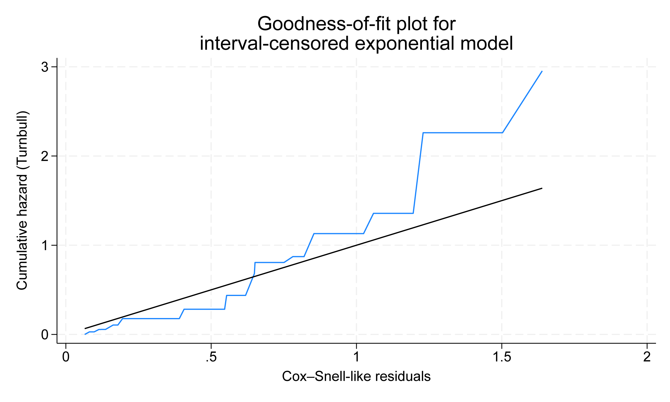
Comparing this GOF plot with the one above, we can see that the Weibull model fits our data better than the exponential model.
References
Aalen, O. O. 1978. Nonparametric inference for a family of counting processes. Annals of Statistics 6: 701–726. https://doi.org/10.1214/aos/1176344247.
Cox, D. R., and E. J. Snell. 1968. A general definition of residuals (with discussion). Journal of the Royal Statistical Society, Series B 30: 248–275.
Crowley, J., and M. Hu. 1977. Covariance analysis of heart transplant survival data. Journal of the American Statistical Association 72: 27–36.
Farrington, C. P. 2000. Residuals for proportional hazards models with interval-censored survival data. Biometrics 56: 473–482.
Finkelstein, D. M., and R. A. Wolfe. 1985. A semiparametric model for regression analysis of interval-censored failure time data. Biometrics 41: 933–945.
Kaplan, E. L., and P. Meier. 1958. Nonparametric estimation from incomplete observations. Journal of the American Statistical Association 53: 457–481.
Nelson, W. 1972. Theory and applications of hazard plotting for censored failure data. Technometrics 14: 945–966.
Turnbull, B. W. 1976. The empirical distribution function with arbitrarily grouped, censored and truncated data. Journal of the Royal Statistical Society, Series B 38: 290–295.

