Numerical integration is used in many computations of integrals when the analytic solutions are not available or difficult to calculate. Vectorized numerical integration approximates a vector of univariate numerical integrations simultaneously.
Mata’s new class, QuadratureVec(), is functionally the same as Quadrature(), except that it handles a vector of integration problems more conveniently. More precisely, QuadratureVec() approximates a vector of univariate integrals numerically by the adaptive Gauss–Kronrod method (the adaptive Simpson method is also provided for comparison).
QuadratureVec() is used in the same way as Quadrature() in only four steps, namely, creating an instance of the class QuadratureVec(), specifying the evaluator functions, setting the limits, and performing the computations.
Let’s see it work
The new Mata class QuadratureVec() is created for the storage and computation of vectorized numerical integration.
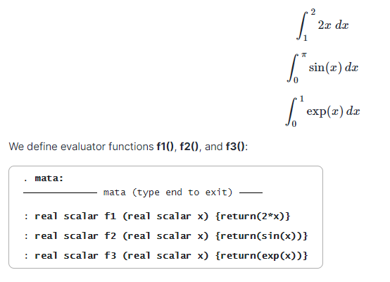
Here is an example to approximate the following three integrals:

Having defined the evaluator functions, we follow the four steps that are required each time we use the QuadratureVec() class. First, we create an instance q of the QuadratureVec() class:
: q = QuadratureVec()
Second, we use setEvaluator() to point to the evaluator functions, defined as the column vector evaluator:
: evaluator = (&f1() \ &f2() \ &f3())
: q.setEvaluator(evaluator)
Third, we use setLimits() to specify the lower and upper limits, defined as limits:
: limits = ((1, 2) \ (0,pi()) \ (0,1))
: q.setLimits(limits)
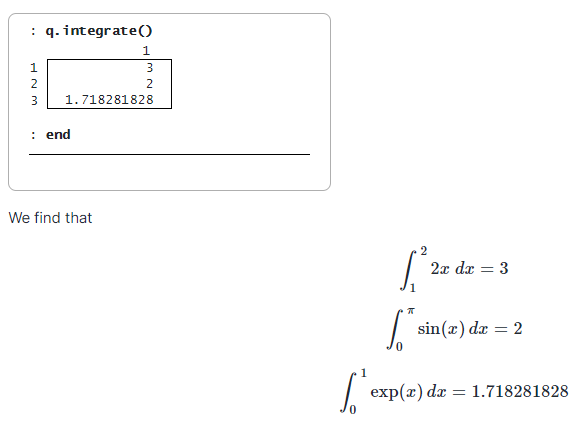
Fourth, we use integrate() to compute the approximations:


