Let’s see it work

We illustrate lasso cox with an example that predicts the risk of death for stage I lung adenocarcinoma patients. Lung adenocarcinoma is one of the most common non-small cell lung cancers.

Stage I adenocarcinoma indicates that the tumor size is relatively small and the cancer has not spread to other distant organs. Stage I adenocarcinoma patients have varied survival outcomes even though they are in the early cancer-development stage. For example, Yu et al. (2016) show that, in one cohort, more than 50% of stage I adenocarcinoma patients died within 5 years after the initial diagnosis, while about 15% of the patients survived for more than 10 years.

Histopathology image features are used for prognostic analysis. We can use lasso cox to extract the top histopathology image features that distinguish short-term and long-term survivors.

We have a fictional survival dataset (lungcancer.dta) inspired by Yu et al. (2016). The variable t records either the time of death or censoring in months for stage I adenocarcinoma lung cancer patients. The indicator variable died is 1 or 0 if the patient died or is censored, respectively. There are 500 histopathology image features, histfeature1 to hisfeature500, and only 250 patients. The analysis aims to classify a new patient into a low-risk or high-risk group, given the histopathology image features.

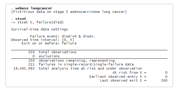
We first load the dataset and then type stset to show that it has already been stset.

Next, we split the full sample into training and testing data. The training data will be used for estimation, and the testing data will be used to measure the prediction performance.

We use splitsample to split the data into two parts. We use the generate(group) option to create a new variable, group, that equals 1 if it belongs to the training data or 0 to the testing data. The split(0.6 0.4) option specifies that 60% of the entire data are used as training data and 40% as testing data. To make the results reproducible, we specify the rseed() option.

. splitsample, generate(group) split(0.6 0.4) rseed(12345)

For later use, we save the training data as lungcancer_training.dta and the testing data as lungcancer_testing.dta.

. preserve

. keep if group == 1
(100 observations deleted)

. save lungcancer_training, replace
file lungcancer_training.dta not found
file lungcancer_training.dta saved

. restore

. preserve

. keep if group == 2
(150 observations deleted)

. save lungcancer_testing, replace
file lungcancer_testing.dta not found
file lungcancer_testing.dta saved

. restore

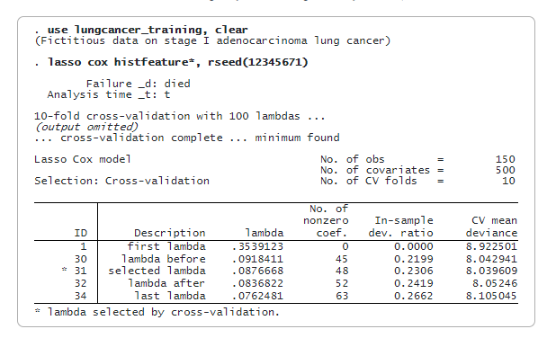
We now fit a lasso cox model using only the training data. By default, we use cross-validation. We specify rseed() for reproducibility.

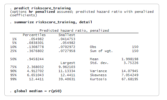
lasso cox selects 48 of the 500 features. We can now predict the penalized relative-hazard ratio (variable riskscore_training) and evaluate risk scores. We will use the median of riskscore_training as a threshold to classify a patient as low risk or high risk. We store the median value in a global macro (median) for later use.

We now use the testing data to validate the model. First, we predict the penalized hazard ratio (variable riskscore_testing) in the testing sample. Then, we compare riskscore_testing with the median of the hazard ratio obtained in the training data ($median). The patient is labeled high risk if the predicted risk score is greater than or equal to the median. The patient is classified as low risk if the predicted risk score is less than the median.

. use lungcancer_testing, clear
(Fictitious data on stage I adenocarcinoma lung cancer)

. predict riskscore_testing
(options hr penalized assumed; predicted hazard ratio with penalized
coefficients)

. generate byte risk = (riskscore_testing >= $median)

. label define risk_lb 1 "High risk" 0 "Low risk"

. label values risk risk_lb

To evaluate the effectiveness of risk classification, we first look at the Kaplan–Meier plot, which plots the survival curve for both low-risk and high-risk groups.

. sts graph, by(risk)

The graph shows that the predicted high-risk patients have a more steeply falling survival curve than the predicted low-risk patients. To confirm this conjecture, we do a log-rank test.

The log-rank test rejects the hypothesis that the predicted low-risk and high-risk patients have the same survival functions. Both the Kaplan–Meier plot and the log-rank test show that using the predicted hazard ratios’ median can effectively distinguish a low-risk patient from a high-risk patient. We can now make prognostic predictions given new data.

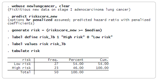
The dataset (newlungcancer.dta) contains histopathology image features for some new stage I adenocarcinoma patients, and we do not observe their survival time yet because they are still alive. Based on the prediction model from lasso cox, we want to classify these new patients as low risk or high risk. To achieve this objective, we need to predict only the new patients’ hazard ratios and compare them with the median level of risk score obtained in the training data.

The table of the predicted risk level shows that 27 patients are classified as low risk, while 23 patients are classified as high risk.

Reference

Yu, K., C. Zhang, G. J. Berry, R. B. Altman, C. Ré, D. L. Rubin, and M. Snyder. 2016. Predicting non-small cell lung cancer prognosis by fully automated microscopic pathology image features. Nature Communications 7(12474).