Launching Version 12.3 of Wolfram Language & Mathematica
Look What We Made in Five Months!

We released Version 12.2 on December 16, 2020. And today, just five months later, we’re releasing Version 12.3. There are some breakthroughs and major new directions in 12.3. But much of what’s in 12.3 is just about making Wolfram Language and Mathematica better, smoother and more convenient to use. Things are faster. More “But what about ___?” cases are handled. Big frameworks are more completely filled out. And there are lots of new conveniences.
There are also the first pieces of what will become large-scale structures in the future. Early functions—already highly useful in their own right—that will in future releases be pieces of major systemwide frameworks.
One way to assess a release is to talk about how many new functions it contains. For Version 12.3 that number is 111 (or about 5 new functions per development-week). It’s a very impressive level of R&D productivity. But particularly for 12.3 it’s just part of the story; there are also 1190 bug fixes (about a quarter for externally reported bugs), and 105 substantially updated and enhanced functions.
Incremental releases are part of our commitment to open development. We’ve also been sharing more kinds of functionality in open-source form (including more than 300 new functions in the Wolfram Function Repository). And we’ve been doing our unique thing of livestreaming our internal design processes. For Version 12.3 it’s once again possible to see just where and how design decisions were made, and the reasoning behind them. And we’ve also had great input from our community (often in real time during livestreams)—that has significantly enhanced the Version 12.3 that we are delivering today.
By the way, when we say “Version 12.3” of Wolfram Language and Mathematica we mean desktop, cloud and engine: all three versions are being released today.
Lots of Little New Conveniences
Version 12.3 has our latest batch of conveniences, scattered across many parts of the language. A new dynamic that’s emerged in this version is functions that have essentially been “prototyped” in the Wolfram Function Repository, and then “upgraded” to be built into the system.
Here’s a first example of a new convenience function: SolveValues. The function Solve—originally introduced in Version 1.0—has a very flexible way of representing its results, that allows for different numbers of variables, different numbers of solutions, etc.
|

|
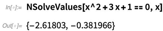
By the way, there’s also an NSolveValues that gives approximate numerical values:
 |
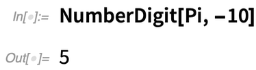
Another example of a new convenience function is NumberDigit. Let’s say you want the 10th digit of π. You can always use RealDigits and then pick out the digit you want:
 |
But now you can also just use NumberDigit (where now by “10th digit” we’re assuming you mean the coefficient of 10-10):
 |
Back in Version 1.0, we just had Sort. In Version 10.3 (2015) we added AlphabeticSort, and then in Version 11.1 (2017) we added NumericalSort. Now in Version 12.3—to round out this family of default types of sorting—we’re adding LexicographicSort. The default sorting sort (as produced by Sort) is:

|
But here’s true lexicographic order, like you would find in a dictionary:

Another small new function in Version 12.3 is StringTakeDrop:
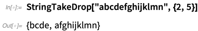
|
Having this as a single function makes it easier to use in functional programming constructs like this:
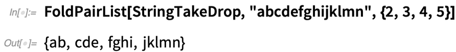 |
It’s always an important goal to make “standard workflows” as straightforward as possible. For example, in handling graphs we’ve had VertexOutComponent since Version 8.0 (2010). It gives a list of the vertices that can be reached from a given vertex. And for some things that’s exactly what one wants. But sometimes it’s much more convenient to get the subgraph (and in fact in the formalism of our Physics Project that subgraph—that we view as a “geodesic ball”—is a rather central construct). So in Version 12.3 we’ve added VertexOutComponentGraph:
 |
Another example of a small “workflow improvement” is in HighlightImage. HighlightImage typically takes a list of regions of interest to highlight in the image. But functions like MorphologicalComponents don’t just make lists of regions in an image; instead they produce a “label matrix” that puts numbers to label different regions in an image. So to make the HighlightImage workflow smoother, in Version 12.3 we let it directly use a label matrix, assigning different colors to the differently labeled regions:
 |
One thing we work hard to ensure in the Wolfram Language is coherence and interoperability. (And in fact, we have a whole initiative around this that we call “Language Completeness & Consistency”, whose weekly meetings we regularly livestream.) One of the various facets of interoperability is that we want functions to be able to “eat” any reasonable input and turn it into something they can “naturally” handle.
And as a small example of this, something we added in Version 12.3 is automatic conversion between color spaces. Red by default means the RGB color red (RGBColor[1,0,0]). But now
 |
means turns that red into red in hue space:
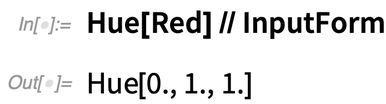
|
Let’s say you’re running a long computation. You often want to get some indication of the progress that’s being made. In Version 6.0 (2007) we added Monitor, and in subsequent versions we’ve added automatic built-in progress reporting for some functions, for example NetTrain. But now we have an initiative underway to systematically add progress reporting for all sorts of functions that can end up doing long computations. ($ProgressReporting = False globally switches it off.)
 |
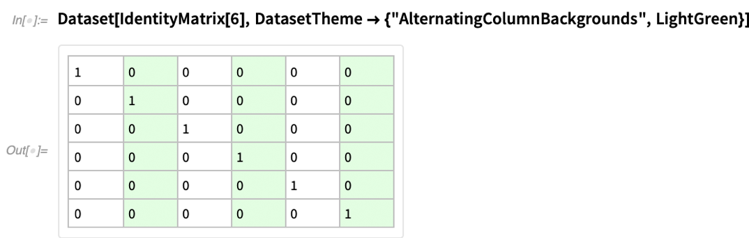
We work hard in Wolfram Language to make sure that we pick good defaults, for example for how to display things. But sometimes you have to tell the system what kind of “look” you want. And in Version 12.3 we’ve added the option DatasetTheme to specify “themes” for how Dataset objects should be displayed.
Underneath, each theme is just setting specific options, which you could set yourself. But the theme is “bank switching” options in a convenient way. Here’s a basic dataset with default formatting:
 |
Here it is looking more “lively” for the web:
 |
You can give various “theme directives” too:
 |
As well as additional hints:
 |
I’m not sure why we didn’t think of it before, but in Version 11.3 (2018) we introduced a very nice “user interface innovation”: Iconize. And in Version 12.3 we’ve added another piece of polish to iconization. If you select a piece of an expression, then use Iconize in the context (“right-click”) menu, an appropriate subpart of the expression will get iconized, even if the selection you made might have included an extra comma, or been something that can’t be a strict subpart of the expression:
 |
Let’s say you generate an object that takes a lot of memory to store:
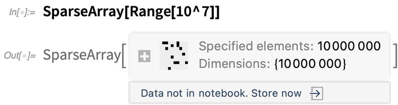 |
By default, the object is kept in your kernel session, but it’s not stored directly in your notebook—so it won’t persist after you end your current kernel session. In Version 12.3 we’ve added some options for where you can store the data:
 |
One important area where we put lots of effort into making things “just work” is in importing and exporting of data. The Wolfram Language now supports about 250 external data formats, with for example new statistical data formats like SAS7BDAT, DTA, POR and SAV being added in Version 12.3.
Lots of Things Got Faster
Here’s a computation with Around:
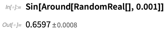 |
In Version 12.2 doing this 10,000 times takes about 1.3 seconds on my computer:
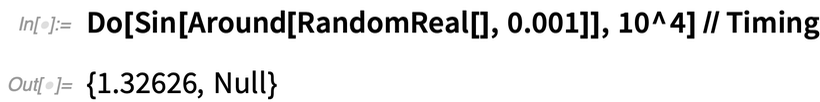 |
In Version 12.3, it’s roughly 100 times faster:
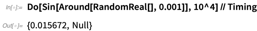 |
There are lots of different reasons that things got faster in Version 12.3. In the case of Permanent, for example, we were able to use a new and much better algorithm. Here it is in 12.2:
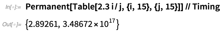 |
And now in 12.3:
 |
One more example is Rasterize, which in Version 12.3 is typically 2 to 4 times faster than in Version 12.2. The reason for this speedup is somewhat subtle. Back when Rasterize was first introduced in Version 6.0 (2007) data transfer speeds between processes were an issue, and so it was a good optimization to compress any data being transferred. But today transfer speeds are much higher, and we have better optimized array data structures—and so compression no longer makes sense, and removing it (together with other codepath optimization) allows Rasterize to be significantly faster.
An important advance in Version 12.1 was the introduction of DataStructure, allowing direct use of optimization data structures (implemented through our new compiler technology). Version 12.3 introduces several new data structures. There’s “ByteTrie” for fast prefix-based lookups (think Autocomplete and GenomeLookup), and there’s “KDTree” for fast geometric lookups (think Nearest). There’s also now “ImmutableVector“, which is basically like an ordinary Wolfram Language list, except that it’s optimized for fast appending.
In addition to speed improvements in the computational kernel, Version 12.3 has user interface speed improvements too. Particularly notable is significantly faster rendering on Windows platforms, achieved by using DirectWrite and making use of GPU capabilities.
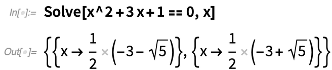
Pushing the Math Frontier
For Version 12.3 let’s talk first about symbolic equation solving. Back in Version 3 (1996) we introduced the idea of implicit “Root object” representations for roots of polynomials, allowing us to do exact, symbolic computations even without “explicit formulas” in terms of radicals. Version 7 (2008) then generalized Root to also work for transcendental equations.
What about systems of equations? For polynomials, elimination theory means that systems really aren’t a different story from individual equations; the same Root objects can be used. But for transcendental equations, this isn’t true anymore. But for Version 12.3 we’ve now figured out how to generalize Root objects so they can work with multivariate transcendental roots:
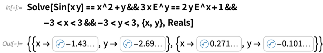 |
And because these Root objects are exact, they can for example be evaluated to any precision:
 |
In Version 12.3 there are also some new equations, involving elliptic functions, where exact symbolic results can be given, even without Root objects:
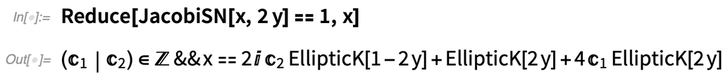 |
A major advance in Version 12.3 is being able to solve symbolically any linear system of ODEs (ordinary differential equations) with rational function coefficients.
Sometimes the result involves explicit mathematical functions:
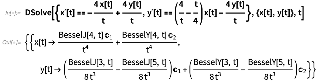 |
Sometimes there are integrals—or differential roots—in the results:
 |
Another ODE advance in Version 12.3 is full coverage of linear ODEs with q-rational function coefficients, in which variables can appear explicitly or implicitly in exponents. The results are exact, though they typically involve differential roots:
 |
What about PDEs? For Version 12.2 we introduced a major new framework for modeling with numerical PDEs. And now in Version 12.3 we’ve produced a whole 105-page monograph about symbolic solutions to PDEs:

|
|
Now it can be solved exactly and symbolically as well:
 |
In addition to linear PDEs, Version 12.3 extends the coverage of special solutions to nonlinear PDEs. Here’s one (with 4 variables) that uses Jacobi’s method:
 |
Something added in 12.3 that both supports PDEs and provides new functionality for signal processing is bilateral Laplace transforms (i.e. integrating from –∞ to +∞, like a Fourier transform):
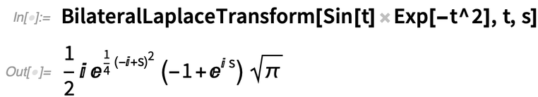 |
Back in Version 3 (1996) we introduced MeijerG which dramatically expanded the range of definite integrals that we could do in symbolic form. MeijerG is defined in terms of a Mellin–Barnes integral in the complex plane. It’s a small change in the integrand, but it’s taken 25 years to unravel the necessary mathematics and algorithms to bring us now in Version 12.3 FoxH.
FoxH is a very general function—that encompasses all hypergeometric pFq and Meijer G functions, and much beyond. And now that FoxH is in our language, we’re able to start the process of expanding our integration and other symbolic capabilities to make use of it.
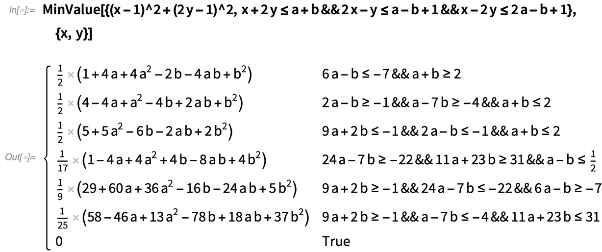
Symbolic Optimization Breakthrough
 |
 |
In typical convex optimization computations not involving symbolic parameters one aims only for approximate numerical results, and it wasn’t clear whether there was any general method for getting exact numerical results. But for Version 12.3 we’ve found one, and we’re now able to give exact numerical results which you can, for example, evaluate to any precision you want.
Here’s a geometric optimization problem—which can now be solved exactly in terms of transcendental root objects:
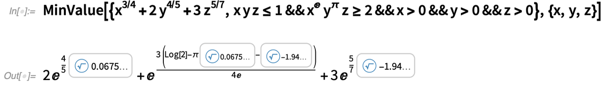 |
Given such an exact solution, it’s now possible to do numerical evaluation to any precision:
 |
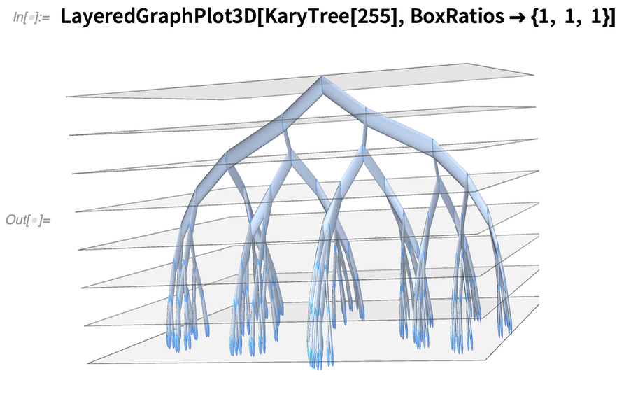
More with Graphs
In Version 12.3 we’ve continued to expand that functionality. Here, for example, is a new 3D visualization function for graphs:
 |
And here’s a new 3D graph embedding:
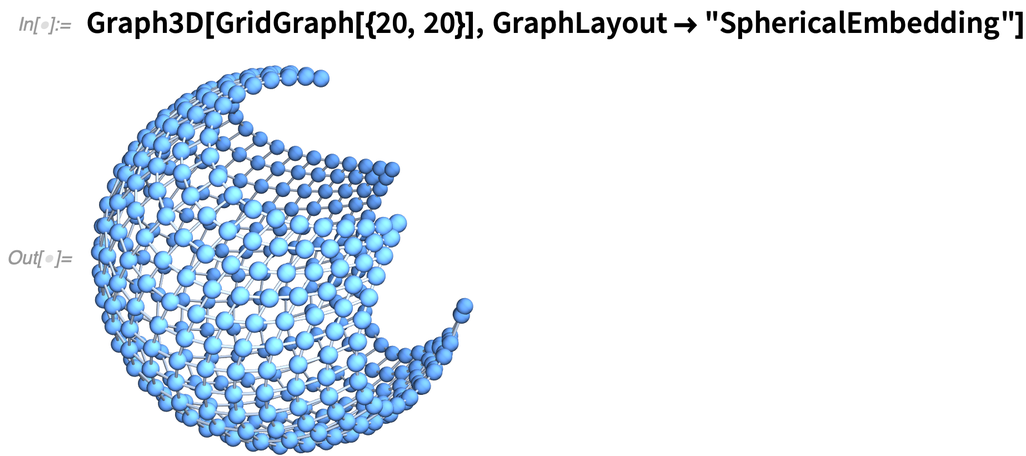 |
We’ve been able to find spanning trees in graphs since Version 10 (2014). In Version 12.3, however, we’ve generalized FindSpanningTree to directly handle objects—like geo locations—that have some kind of coordinates. Here’s a spanning tree based on the positions of capital cities in Europe:
 |
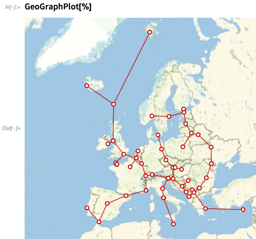 |
By the way, in a “geo graph” there are “geo” ways to route the edges. For example, you can specify that they follow (when possible) driving directions (as provided by TravelDirections):
 |
Euclid Meets Descartes, and More
Given three symbolically specified points, GeometricTest can give the algebraic condition for them to be collinear:
 |
For the particular case of collinearity, there’s a specific function for doing the test:
 |
But GeometricTest is much more general in scope—supporting more than 30 kinds of predicates. This gives the condition for a polygon to be convex:
 |
And this gives the condition for a polygon to be regular:
 |
And here’s the condition for three circles to be mutually tangent (and, yes, that ∃ is a little “post Descartes”):
 |
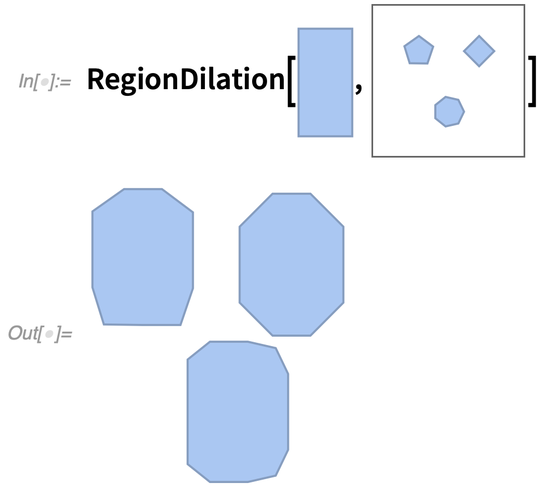
Version 12.3 also has enhancements to core computational geometry. Most notable are RegionDilation and RegionErosion, that essentially convolve regions with each other. RegionDilation effectively finds the whole (“Minkowski sum”) “union region” obtained by translating one region to every point in another region.
Why is this useful? It turns out there are lots of reasons. One example is the “piano mover problem” (AKA the robot motion planning problem). Given, say, a rectangular shape, is there a way to maneuver it (in the simplest case, without rotation) through a house with certain obstacles (like walls)?
Basically what you need to do is take the rectangular shape and “dilate the room” (and the obstacles) with it:
 |
Then if there’s a connected path “left over” from one point to another, then it’s possible to move the piano along that path. (And of course, the same kind of thing can be done for robots in a factory, etc. etc.)
RegionDilation is also useful for “smoothing out” or “offsetting” shapes, for example, for CAD applications:
 |
At least in simple cases, one can “go Descartes” with it, and get explicit formulas:
 |
And, by the way, this all works in any number of dimensions—providing a useful way to generate all sorts of “new shapes” (like a cylinder is the dilation of a disk by a line in 3D).
Yet More Visualization
Here’s a 3D random walk rendered with ListLinePlot3D:
 |
If you give multiple lists of data, ListLinePlot3D plots them each separately:
 |
We first introduced plotting of vector fields in Version 7.0 (2008), with functions like VectorPlot and StreamPlot—that were substantially enhanced in Versions 12.1 and 12.2. In Version 12.3 we’re now adding StreamPlot3D (as well as ListStreamPlot3D). Here’s a plot of streamlines for a 3D vector field, colored by field strength:

Axes work a bit like arrows: first you give the “core structure”, then you say how to annotate it. Here’s an axis that is linearly labeled from 0 to 100 on a line:


Golden Knots, and Other Material Matters


The story of modeling light interacting with surfaces—and “physically based rendering”—is a complicated one, that Version 12.3 has a whole monograph about:

Trees!
The fundamental object is Tree:

There are a variety of “*Tree” functions for constructing trees, and “Tree*” functions for converting trees to other things. RulesTree, for example, constructs a tree from a nested collection of rules:


When we were designing Tree we at first thought we’d have to have separate symbolic representations of whole trees, subtrees and leaf nodes. But it turned out that we were able to make an elegant design with Tree alone. Nodes in a tree typically have the form Tree[payload, {child1, child2, …}] where the childi are subtrees. A node doesn’t necessarily have to have a payload, in which case it can just be given as Tree[{child1, child2, …}]. A leaf node is then Tree[expr, None] or Tree[None].
One very nice feature of this design is that trees can immediately be constructed from subtrees just by nesting expressions:


Dates, Times and How Fast Is the Earth Turning?
Here’s a date with the standard conventions used in Swedish:


aIn Version 12.3, there’s a new detailed specification for how date formats should be constructed:


We introduced sidereal (star-based) time in Version 10.0 (2014):


This tells how much longer than 24 hours the day currently is:


The Leading Edge of Machine Learning & Neural Nets
Train a predictor to predict “wine quality” from the chemical content of a wine:


A subtle but important issue in machine learning is calibrating the “confidence” of classifiers. If a classifier says that certain images have 60% probability to be cats, does this mean that 60% of them actually are cats? A raw neural net won’t typically get this right. But one can get closer by recalibrating probabilities using a calibration curve. And in Version 12.3, in addition to automatic recalibration, functions like Classify support the new RecalibrationFunction option that allows you to specify how the recalibration should be done.
An important part of our machine learning framework is in-depth symbolic support for neural nets. And we’ve continued to put the latest neural nets from the research literature into our Neural Net Repository, making them immediately accessible in our framework using NetModel.
In Version 12.3 we’ve added a few extra features to our framework, for example “swish” and “hardswish” activation functions for ElementwiseLayer. “Under the hood” a lot has been going on. We’ve enhanced ONNX import and export, we’ve greatly streamlined the software engineering of our MXNet integration, and we’ve almost finished a native version of our framework for Apple Silicon (in 12.3.0 the framework runs through Rosetta).
We’re always trying to make our machine learning framework as automated as possible. And in achieving this, it’s been very important that we’ve had so many curated net encoders and decoders that you can immediately use on different kinds of data. In Version 12.3 an extension to this is the use of an arbitrary feature extractor as a net encoder, that can be trained as part of your main training process. Why is this important? Well, it gives you a trainable way to feed into a neural net arbitrary collections of data of different kinds, even though there’s no pre-defined way of even knowing how the data can be turned into something like an array of numbers suitable for input to a neural net.
In addition to providing direct access to state-of-the-art machine learning, the Wolfram Language has an increasing number of built-in functions that make powerful internal use of machine learning. One such function is TextCases. And in Version 12.3 TextCases has become significantly stronger, especially in supporting less common text content types, like “Protein” and “BoardGame“:

New in Video
A major group of new capabilities in 12.3 revolve around programmatic video generation. There are three basic new functions: FrameListVideo, SlideShowVideo and AnimationVideo.
FrameListVideo takes a raw list of images, and assembles a video by treating them as successive raw frames. SlideShowVideo similarly takes a list of images, but now it creates a “slide show video” in which each image is displayed for a specified duration. Here, for example, each image is displayed in the video for 1 second:

AnimationVideo doesn’t take existing images; instead it takes an expression and then evaluates it “Manipulate-style” for a range of values of a parameter. (In effect, it’s like a video-making analog of Animate.)


So, for example, here’s me green-screen composited with the stream above:

Version 12.3 also adds some new video-editing capabilities. VideoTimeStretch lets you “warp time” in a video by any specified function. VideoInsert lets you insert a video clip into a video, and VideoReplace lets you replace part of a video with another one.
One of the best things about video in the Wolfram Language is that it can immediately be analyzed using all of the tools in the language. This includes machine learning, and in Version 12.3 we’ve started the process of allowing videos to be encoded for neural net computation. Version 12.3 includes a simple frame-based net encoder for videos, as well as a couple of built-in feature extractors. More will be coming soon, including a variety of video processing and analysis nets in the Wolfram Neural Net Repository.
More in Chemistry
In Version 12.3, for example, there are new properties for Molecule, like “TautomerList” (possible reconfigurations in solution):


Closing the Loop for Control Systems
Let’s start by importing a model that was created in Wolfram System Modeler. In this particular case, it’s a simple model for a submarine:


So given the underlying system model, how can we design that controller? Well, in Version 12.3 we’ve managed to get it down to just a couple of functions. First we give the model and parameters that are going to be controlled, and specify our design goal by giving the eigenvalues we want:


So how did this work? Well, as is typical in this type of control systems design, we first found a linearization of the underlying model, appropriate for the domain in which we were going to be operating:


It’s Going to Get Easier to Type Code in Notebooks
So this means for example that instead of your code looking this


But if you’re dealing with [[ … ]] you can’t just do this kind of “local replacement” without the potential for confusion with some ]] showing up as 〛 while others break apart into ]] as a result of routine editing.
In Version 12.3 what we’re doing is not to make replacements at all, but instead just to render specified sequences of characters (like ]]) in special ways. The result is that we can support very general “ligature-like” behavior, and that backspacing will always exactly reverse characters that were entered.
AutoOperatorRenderings will make code you type look nicer and be easier to read. But there’s a second, more significant change in the way you enter code that’s now available in Version 12.3. It’s still rather experimental, so it hasn’t been turned on by default, but you can explicitly turn it on if you want, just by evaluating

So that means that if you type

So what happens to your old typing habits? Well, you can still use them. Because you can enter ] to “type through” the closing ]. And that means you’re typing the exact same characters as before. But the important point is that you don’t need to. The ] is already there for you.
Why is this important? Basically because it means you don’t have to think about matching your delimiters anymore. It’s done automatically for you. Ever since Version 3.0 (1996) we’ve had syntax coloring that indicates when delimiters haven’t been closed—and to suggest that you should close them. But now the closing will just happen automatically. And in particular that means that expressions you’re typing will always “look complete”, and won’t have all kinds of structural changes happening as you enter each character.
Needless to say, this is all a lot trickier than it might at first appear. Let’s say you’ve already entered a complicated expression, and now you add an opening delimiter inside it, or, worse, several opening delimiters. Where do the closing delimiters go? How much of the code that’s already there should they enclose? Sometimes it’s fairly obvious, but sometimes it’s not. You can always delete an inappropriately added closing delimiter, but we’re working hard to use the appropriate heuristics to either add the closing delimiter in the right place, or not add it at all.
What’s Wrong with That Code? Code Analysis & Assistance
We’ve had things like syntax coloring and ^ for missing arguments for decades. And these are extremely useful. But what we want is something more global. Something not so much like spellchecking as like being able to say whether a piece of text means the right thing.
One might think that there’s a kind of philosophical problem with this. In the Wolfram Language any piece of code—so long as it’s syntactically correct—is a symbolic expression which at some level means something. The question is whether that “something” is what you want. And the point is that by knowing the typical structure of “correct code” it’s often possible to make a very good guess. And that’s what our new code analysis system does.
Say you have this simple piece of code:


Here’s a marginally more complicated example:

Does Code Analysis catch real errors? Yes, and we’ve got evidence for that, because we’ve run it on our internal code, as well as on examples in our documentation. For example, in Version 12.2 the documentation for FitRegularization contained the example:


Advances in the Compiler: Portability and Librarying
In Version 12.3 we took an important step to make the workflow for this easier. Let’s say you compile a very simple function:
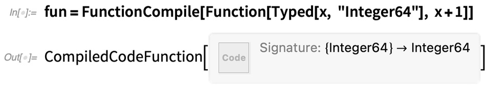
What is that output? Well, in Version 12.3 it’s a symbolic object that contains raw low-level code:

But an important point is that everything is right there in this symbolic object. So you can just pick it up and use it:
 |
There’s a slight catch, however. By default, FunctionCompile will generate raw low-level code for the type of computer on which you’re running. But if you take the resulting CompiledCodeFunction to another type of computer, it won’t be able to use the low-level code. (It keeps a copy of the original expression before compilation, so it can still run, but won’t have the efficiency advantage of compiled code.)
In Version 12.3, there’s a new option to FunctionCompile: TargetSystem. And with TargetSystem → All you can tell FunctionCompile to create cross-compiled low-level code for all current systems:
 |
Needless to say, it’s slower to do all that compilation. But the result is a portable object that contains low-level code for all current platforms:
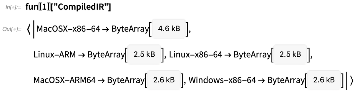 |
So if you have a notebook—or a Wolfram Function Repository entry—that contains this kind of CompiledCodeFunction you can send it to anyone, and it will automatically run on their system.
There are a few other subtleties to this. The low-level code created by default in FunctionCompile is actually LLVM IR (intermediate representation) code, not pure machine code. The LLVM IR is optimized for each particular platform, but when the code is loaded on the platform, there’s the small additional step of locally converting to actual machine code. You can use UseEmbeddedLibrary → True to avoid this step, and pre-create a complete library that includes your code.
This will make it slightly faster to load compiled code on your platform, but the catch is that creating a complete library can only be done on a specific platform. We’ve built a prototype of a cloud-based compilation-as-a-service system, but it’s not yet clear if the speed improvement is worth the trouble.
Another new compiler feature for Version 12.3 is that FunctionCompile can now take a list or association of functions that are compiled together, optimizing with all their interdependencies.
The compiler continues to get stronger and broader, with more and more functions and types (like “Integer128”) being supported. And to support larger-scale compilation projects, something added in Version 12.3 is CompilerEnvironmentObject. This is a symbolic object that represents a whole collection of compiled resources (for example defined by FunctionDeclaration) that act like a library and can immediately be used to provide an environment for additional compilation that is being done.
Shell, Java, …: New Built-in External Connections
First, there’s the shell. Back in Version 1.0, there was the notion of “shell escapes”: type ! at the beginning of a line, and everything after it would be sent to your operating system shell. A third of a century later, it’s a bit more polished and sophisticated, though it’s the same basic idea.
Type > in a notebook, and select Shell, then type your shell command:
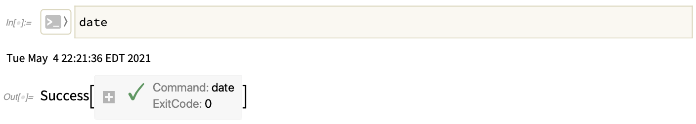 |
The stdout from the shell will be echoed as it’s generated, and then what comes back will be a symbolic object—from which it’s possible to extract things like exit code, or stdout:
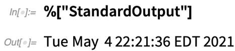 |
In earlier versions, we added capabilities for languages like Python, Julia, R, etc., as well as SQL. In this version, we’re also adding support for Octave (yes, the function names are not great):
 |
But the important point here is that data structures have been connected so that an Octave array comes back as an appropriate expression, in this case a list of lists (containing approximate numbers, because that’s all Octave handles).
By the way, although external language cells in notebooks are nice, you definitely don’t have to use them, and you can use ExternalEvaluate—or ExternalFunction—to do things purely programmatically.
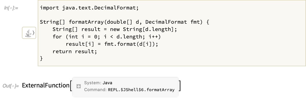
We’ve had tight integration with Java in Wolfram Language through J/Link for more than 20 years. But in Version 12.3 we’ve set things up so that instead of using J/Link’s sophisticated symbolic interface to Java, you can just enter Java code directly in ExternalEvaluate and external language cells:
 |
Basic Java data structures are returned as standard Wolfram Language expressions:
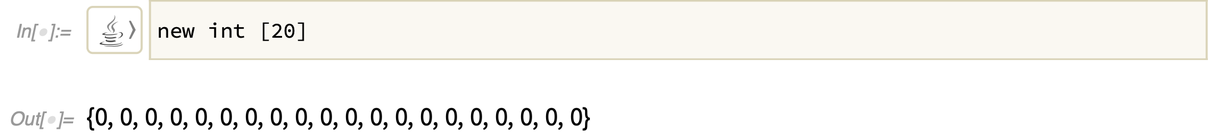 |
Java objects are represented symbolically through J/Link:
 |
Everything interacts seamlessly with J/Link. And for example, you can create Java objects directly using J/Link—that you can subsequently use with Java you enter in an external language cell:

If you define a Java function it gets represented symbolically as an ExternalFunction object:
This particular function takes a list of numbers, and a Java object—of the kind we created above with J/Link:
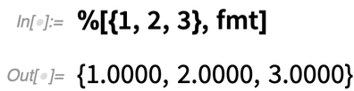
(Yes, this particular operation is extremely easy to do directly in Wolfram Language.)
Blockchain, Storage, Authentication & Cryptography
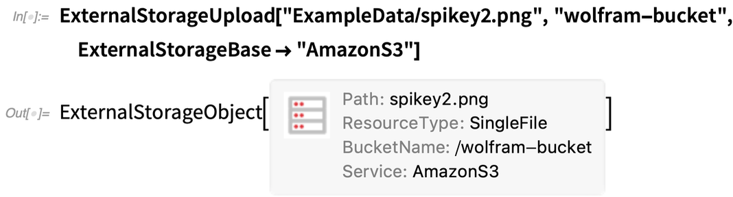
In Version 12.1 we introduced ExternalStorageObject, initially supporting IPFS and Dropbox. In Version 12.3 we’ve added support for Amazon S3 (and, yes, you can store and retrieve a whole bucket of files at a time):
A necessary step in all sorts of external interactions is authentication. And in Version 12.3 we’ve added support for OAuth 2.0 workflows. You create a SecuredAuthenticationKey:

You’ll get a browser window that asks you to log in with your account—and then you’ll be off and running.
For many common external services, we have “pre-packaged” ServiceConnect connections. Often these require authentication. And for OAuth-based APIs (like Reddit or Twitter) we have our WolframConnector app that brokers the external part of the authentication. A new feature of Version 12.3 is that you can also use your own external app to broker that authentication, so you’re not limited by the arrangements made with the external service for the WolframConnector app.
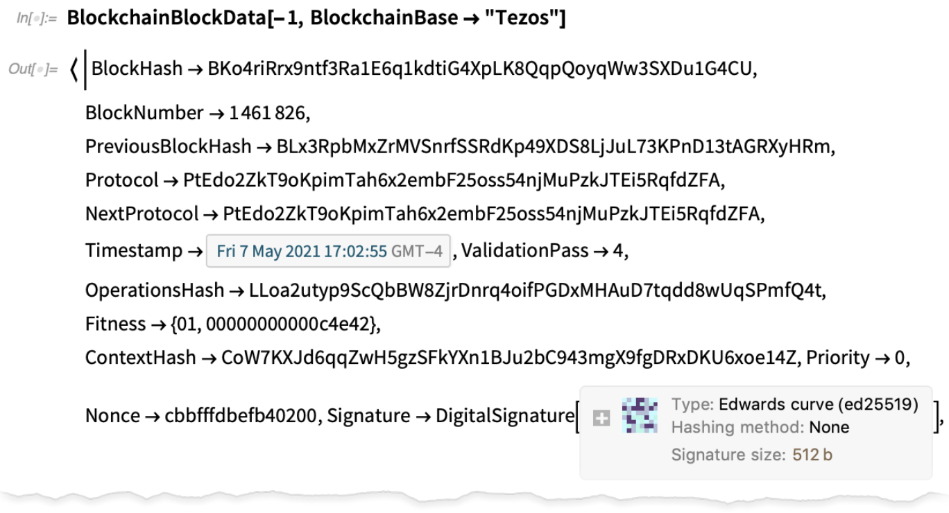
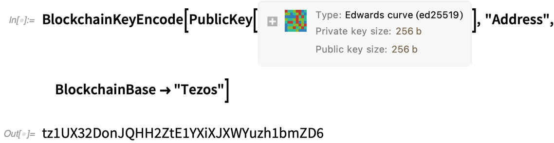
Under the hood for everything we’re talking about here is cryptography. And in Version 12.3 we’ve added some new cryptographic capabilities; in particular we now have support for all elliptic curves in the NIST Digital Signature FIPS 186-4 standard, as well as for Edwards curves that will be part of FIPS 186-5.
We’ve packaged all of this to make it very easy to create blockchain wallets, sign transactions, and encode data for blockchains:

Distributed Computing & Its Management
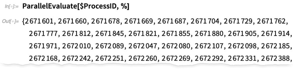
In Version 12.2 we introduced RemoteKernelObject as a symbolic representation of remote Wolfram Language capabilities. Starting in Version 12.2, this was available for one-shot evaluations with RemoteEvaluate. In Version 12.3 we’ve integrated RemoteKernelObject into parallel computation.
Let’s try this for one of my machines. Here’s a remote kernel object that represents a single kernel on it:

Now we can do a computation there, here just asking for the number of processor cores:
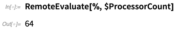
Now let’s create a remote kernel object that uses all 64 cores on this machine:
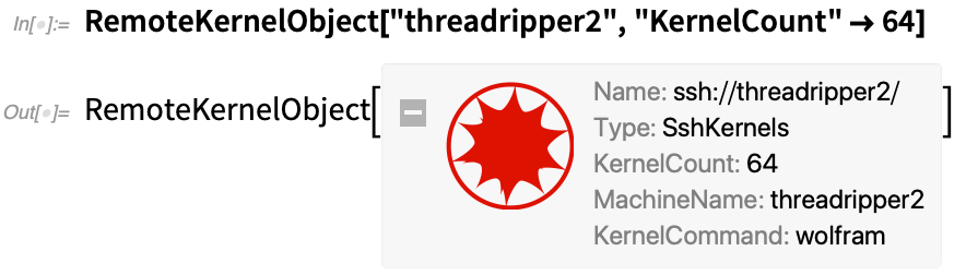
Now I can launch those kernels (and, yes, it’s much faster and more robust than before):
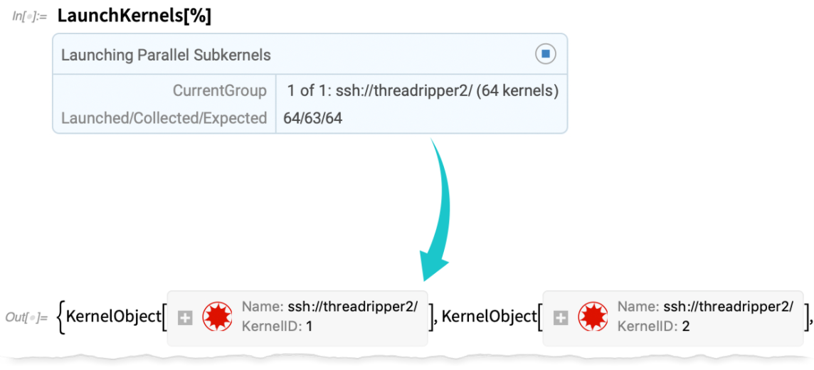
Now I can use this to do parallel computations:
For someone like me who is often involved in doing parallel computations, the streamlining of these capabilities in Version 12.3 will make a big difference.
One feature of functions like ParallelMap is that they’re basically just sending pieces of a computation independently to different processors. Things can get quite complicated when there needs to be communication between processors and everything is happening asynchronously.
The basic science of this is deeply related to the story of multiway graphs and to the origins of quantum mechanics in our Physics Project. But at a practical level of software engineering, it’s about race conditions, thread safety, locking, etc. And in Version 12.3 we’ve added some capabilities around this.
In particular, we’ve added the function WithLock that can lock files (or local objects) during a computation, thereby preventing interference between different processes which attempt to write to the file. WithLock provides a low-level mechanism for ensuring atomicity and thread safety of operations.
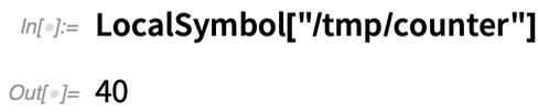
There’s a higher-level version of this in LocalSymbol. Say one sets a local symbol to 0:
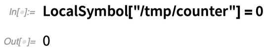
Then launch 40 local parallel kernels (they need to be local so they share files):
Now, because of locking, the counter will be forced to update sequentially on each kernel: