MATHEMATICA V13

Launching Version 13.0 of Wolfram Language + Mathematica

The March of Innovation Continues

by Stephen Wolfram

Just a few weeks ago it was 1/3 of a century since Mathematica 1.0 was released. Today I’m excited to announce the latest results of our long-running R&D pipeline: Version 13 of Wolfram Language and Mathematica. (Yes, the 1, 3 theme—complete with the fact that it’s the 13th of the month today—is amusing, if coincidental.)

It’s 207 days—or a little over 6 months—since we released Version 12.3. And I’m pleased to say that in that short time an impressive amount of R&D has come to fruition: not only a total of 117 completely new functions, but also many hundreds of updated and upgraded functions, several thousand bug fixes and small enhancements, and a host of new ideas to make the system ever easier and smoother to use.

Every day, every week, every month for the past third of a century we’ve been pushing hard to add more to the vast integrated framework that is Mathematica and the Wolfram Language. And now we can see the results of all those individual ideas and projects and pieces of work: a steady drumbeat of innovation sustained now over the course of more than a third of a century:

This plot reflects lots of hard work. But it also reflects something else: the success of the core design principles of the Wolfram Language. Because those are what have allowed what is now a huge system to maintain its coherence and consistency—and to grow ever stronger. What we build today is not built from scratch; it is built on top of the huge tower of capabilities that we have built before. And that is why we’re able to reach so far, automate so much—and invent so much.

In Version 1.0 there were a total of 554 functions altogether. Yet between Version 12.0 and Version 13.0 we’ve now added a total of 635 new functions (in addition to the 702 functions that have been updated and upgraded). And it’s actually even more impressive than that. Because when we add a function today the expectations are so much higher than in 1988—because there’s so much more automation we can do, and so much more in the whole system that we have to connect to and integrate with. And, of course, today we can and do write perhaps a hundred times more extensive and detailed documentation than would have ever fit in the (printed) Mathematica Book of 1988.

The complete span of what’s new in Version 13 relative to Version 12 is very large and impressive. But here I’ll just concentrate on what’s new in Version 13.0 relative to Version 12.3; I’ve written before about Version 12.1, Version 12.2 and Version 12.3.

Don’t Forget Integrals!

Back in 1988 one of the features of Mathematica 1.0 that people really liked was the ability to do integrals symbolically. Over the years, we’ve gradually increased the range of integrals that can be done. And a third of a century later—in Version 13.0—we’re delivering another jump forward. Here’s an integral that couldn’t be done “in closed form ” before, but in Version 13.0 it can:

Any integral of an algebraic function can in principle be done in terms of our general DifferentialRoot objects. But the bigger algorithmic challenge is to get a “human-friendly answer” in terms of familiar functions. It’s a fragile business, where a small change in a coefficient can have a large effect on what reductions are possible. But in Version 13.0 there are now many integrals that could previously be done only in terms of special functions, but now give results in elementary functions. Here’s an example:

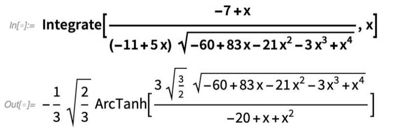
In Version 12.3 the same integral could still be done, but only in terms of elliptic integrals:

Mathematical Functions: A Milestone Is Reached

Back when one still had to do integrals and the like by hand, it was always a thrill when one discovered that one’s problem could be solved in terms of some exotic “special function” that one hadn’t even heard of before. Special functions are in a sense a way of packaging mathematical knowledge: once you know that the solution to your equation is a Lamé function, that immediately tells you lots of mathematical things about it.

In the Wolfram Language, we’ve always taken special functions very seriously, not only supporting a vast collection of them, but also making it possible to evaluate them to any numerical precision, and to have them participate in a full range of symbolic mathematical operations.

When I first started using special functions about 45 years ago, the book that was the standard reference was Abramowitz & Stegun’s 1964 Handbook of Mathematical Functions. It listed hundreds of functions, some widely used, others less so. And over the years in the development of Wolfram Language we’ve steadily been checking off more functions from Abramowitz & Stegun.
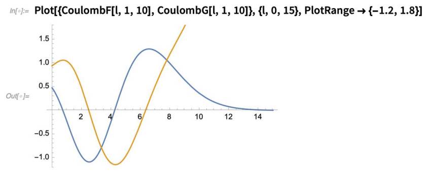
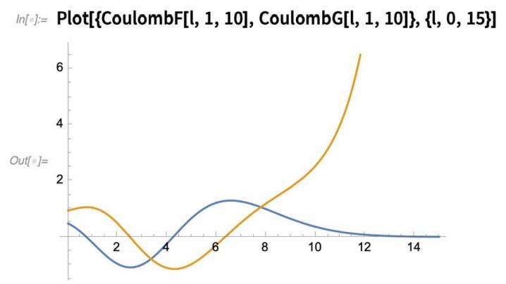
And in Version 13.0 we’re finally done! All the functions in Abramowitz & Stegun are now fully computable in the Wolfram Language. The last functions to be added were the Coulomb wavefunctions (relevant for studying quantum scattering processes). Here they are in Abramowitz & Stegun:

And here’s—as of Version 13—how to get that first picture in Wolfram Language:

Of course there’s more to the story, as we can now see:

Another Kind of Number

One might think that a number is just a number. And that’s basically true for integers. But when a number is a real number the story is more complicated.
Sometimes you can “name” a real number symbolically, say . But most real numbers don’t have “symbolic names”. And to specify them exactly you’d have to give an infinite number of digits, or the equivalent. And the result is that one ends up wanting to have approximate real numbers that one can think of as representing certain whole collections of actual real numbers.

A straightforward way of doing this is to use finite-precision numbers, as in:

Another approach—introduced in Version 12.0—is Around, which in effect represents a distribution of numbers “randomly distributed” around a given number:

When you do operations on Around numbers the “errors” are combined using a certain calculus of errors that’s effectively based on Gaussian distributions—and the results you get are always in some sense statistical.

But what if you want to use approximate numbers, but still get provable results? One approach is to use Interval. But a more streamlined approach now available in Version 13.0 is to use CenteredInterval. Here’s a CenteredInterval used as input to a Bessel function:

You can prove things in the Wolfram Language in many ways. You can use Reduce. You can use FindEquationalProof. And you can use CenteredInterval—which in effect leverages numerical evaluation. Here’s a function that has complicated transcendental roots:

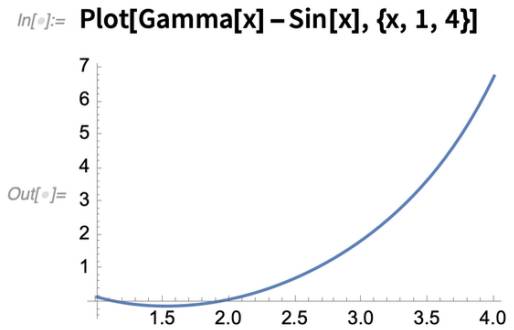
Can we prove that the function is above 0 between 3 and 4? Let’s evaluate the function over a centered interval there:

Now we can check that indeed “all of this interval” is greater than 0:

And from the “worst-case” way the interval was computed this now provides a definite theorem.

As Well As Lots of Other Math…

As in every new version of the Wolfram Language, Version 13.0 has lots of specific mathematical enhancements. An example is a new, convenient way to get the poles of a function. Here’s a particular function plotted in the complex plane:

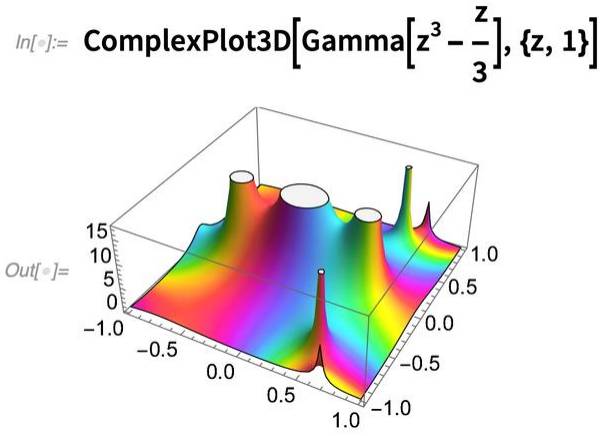
And here are the exact poles (and their multiplicities) for this function within the unit circle:

Now we can sum the residues at these poles and use Cauchy’s theorem to get a contour integral:

Also in the area of calculus we’ve added various conveniences to the handling of differential equations. For example, we now directly support vector variables in ODEs:

Using our graph theory capabilities we’ve also been able to greatly enhance our handling of systems of ODEs, finding ways to “untangle” them into blockdiagonal forms that allow us to find symbolic solutions in much more complex cases than before.

For PDEs it’s typically not possible to get general “closed-form” solutions for nonlinear PDEs. But sometimes one can get particular solutions known as complete integrals (in which there are just arbitrary constants, not “whole” arbitrary functions). And now we have an explicit function for finding these:

Turning from calculus to algebra, we’ve added the function PolynomialSumOfSquaresList that provides a kind of “certificate of positivity” for a multivariate polynomial. The idea is that if a polynomial can be decomposed into a sum of squares (and most, but not all, that are never negative can) then this proves that the polynomial is indeed always nonnegative:

And, yes, summing the squares gives the original polynomial again:

In Version 13.0 we’ve also added a couple of new matrix functions. There’s Adjugate, which is essentially a matrix inverse, but without dividing by the determinant. And there’s DrazinInverse which gives the inverse of the nonsingular part of a matrix—as used particularly in solving differentialalgebraic equations.

More PDE Modeling: Solid & Structural Mechanics

PDEs are both difficult to solve and difficult to set up for particular situations. Over the course of many years we’ve built state-of-the-art finite-element solution capabilities for PDEs. We’ve also built our groundbreaking symbolic computational geometry system that lets us flexibly describe regions for PDEs. But starting in Version 12.2 we’ve done something else too: we’ve started creating explicit symbolic modeling frameworks for particular kinds of physical systems that can be modeled with PDEs. We’ve already got heat transfer, mass transport and acoustics. Now in Version 13.0 we’re adding solid and structural mechanics.

For us a “classic test problem” has been the deflection of a teaspoon. Here’s how we can now set that up. First we need to define our variables: the displacements of the spoon in each direction at each x, y, z point:

Then we need to say what the material parameters of our spoon are. And here we get to make use of our whole knowledgebase, which contains detailed information on many kinds of materials:

Now we’re ready to actually set up and solve the PDE problem:

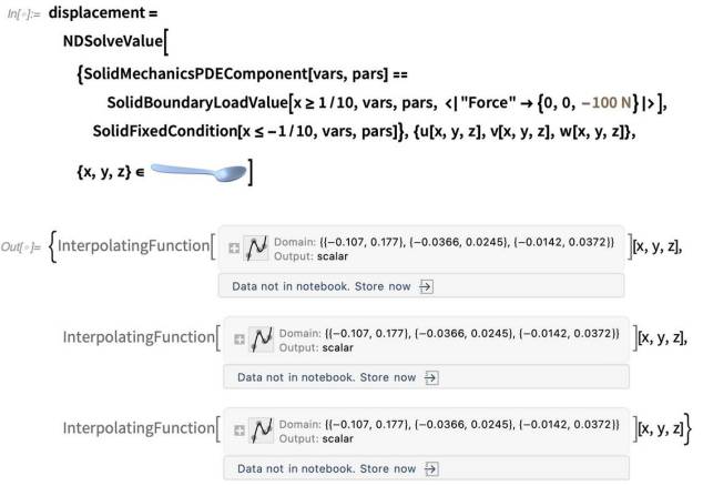
The result is given as a list of interpolating functions for the x, y, z displacements. Now we can use a new Version 13.0 graphics function to immediately visualize this result:

But conveniently packaged in those interpolation functions is also lots more detail about the solution we got. For example, here’s the strain tensor for the spoon, given as a symmetrized array of interpolating functions:

And now we can for example find the maximum 3, 3 component of the strain tensor and the position where it’s achieved:

How about finding the distribution of values of the strain over the spoon? One easy way to do that is just to sample random points in the spoon

and then to make a smoothed histogram of the strains at those points:

(The maximum we saw before is in the tail on the right.) Solid mechanics is a complicated area, and what we have in Version 13 is good, industrial-grade technology for handling it. And in fact we have a whole monograph titled “Solid Mechanics Model Verification” that describes how we’ve validated our results. We are also providing a general monograph on solid mechanics that describes how to take particular problems and solve them with our technology stack.

Making Videos from Images & Videos

In Version 12.3 we released functions like AnimationVideo and SlideShowVideo which make it easy to produce videos from generated content. In Version 13.0 we now also have a collection of functions for creating videos from existing images, and videos. By the way, before we even get to making videos, another important new feature in Version 13.0 is that it’s now possible to play videos directly in a notebook:

This works both on the desktop and in the cloud, and you get all the standard video controls right in the notebook, but you can also pop out the video to view it with an external (say, full-screen) viewer. (You can also now just wrap a video with AnimatedImage to make it into a “GIF-like” frame-based animation.) OK, so back to making videos from images. Let’s say you have a large image:

A good way to “experience” an image like this can be through a “tour video” that visits different parts of the image in turn. Here’s an example of how to do that:

You can zoom as well as pan:

As a more sophisticated example, let’s take a classic “physics image”:

This finds the positions of all the faces, then computes a shortest tour visiting each of them:

Now we can create a “face tour” of the image:

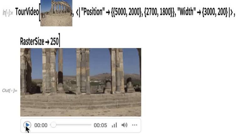
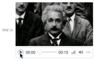
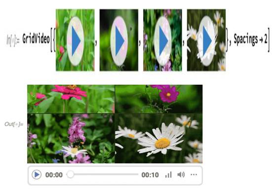
In addition to going from images to videos, we can also go from videos to videos. GridVideo takes multiple videos, arranges them in a grid, and creates a combined new video:

We can also take a single video and “summarize” it as a series of video + audio snippets, chosen for example equally spaced in the video. Think of it as a video version of VideoFrameList. Here’s an example “summarizing” a 75-minute video:

There are some practical conveniences for handling videos that have been added in Version 13.0. One is OverlayVideo which allows you to “watermark” a video with an image, or insert what amounts to a “picture-in-picture” video:

We’ve also made many image operations directly work on videos. So, for example, to crop a video, you just need to use ImageCrop:

Image Stitching

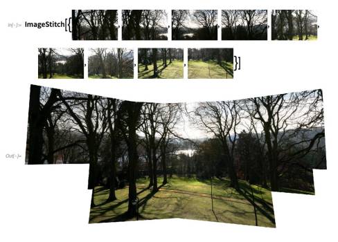
Let’s say you’ve taken a bunch of pictures at different angles—and now you want to stitch them together. In Version 13.0 we’ve made that very easy—with the function ImageStitch:

Part of what’s under the hood in image stitching is finding key points in images. And in Version 13.0 we’ve added two further methods (SIFT and RootSIFT) for ImageKeypoints. But aligning key points isn’t the only thing we’re doing in image stitching. We’re also doing things like brightness equalization and lens correction, as well as blending images across seams.

Image stitching can be refined using options like TransformationClass—which specify what transformations should be allowed when the separate images are assembled.

Trees Continue to Grow

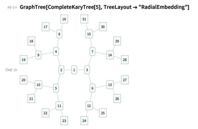
We introduced Tree as a basic construct in Version 12.3. In 13.0 we’re extending Tree and adding some enhancements. First of all, there are now options for tree layout and visualization.

For example, this lays out a tree radially (note that knowing it’s a tree rather than a general graph makes it possible to do much more systematic embeddings):

This adds options for styling elements, with one particular element specified by its tree position being singled out as blue:

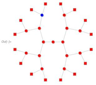
One of the more sophisticated new “tree concepts” is TreeTraversalOrder. Imagine you’re going to “map across” a tree. In what order should you visit the nodes? Here’s the default behavior. Set up a tree:

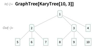
Now show in which order the nodes are visited by TreeScan:

This explicitly labels the nodes in the order they are visited:

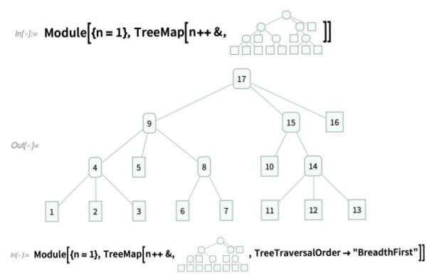
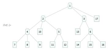
Here’s a slightly more ornate ordering:

Why does this matter? “Traversal order” turns out to be related to deep questions about evaluation processes and what I now call multicomputation. In a sense a traversal order defines the “reference frame” through which an “observer” of the tree samples it. And, yes, that language sounds like physics, and for a good reason: this is all deeply related to a bunch of concepts about fundamental physics that arise in our Physics Project. And the parametrization of traversal order—apart from being useful for a bunch of existing algorithms—begins to open the door to connecting computational processes to ideas from physics, and new notions about what I’m calling multicomputation.

Graph Coloring

The graph theory capabilities of Wolfram Language have been very impressive for a long time (and were critical, for example, in making possible our Physics Project). But in Version 13.0 we’re adding still more.

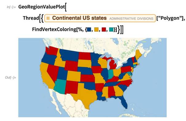
A commonly requested set of capabilities revolve around graph coloring. For example, given a graph, how can one assign “colors” to its vertices so that no pair of adjacent vertices have the same color? In Version 13.0 there’s a function FindVertexColoring that does that:

And now we can “highlight” the graph with those colors:

The classic “graph coloring” problem involves coloring geographic maps. So here, for example, is the graph representing the bordering relations for US states:

Now it’s an easy matter to find a 4-coloring of US states:

There are actually a remarkable range of problems that can be reduced to graph coloring. Another example has to do with scheduling a “tournament” in which all pairs of people “play” each other, but everyone plays only one match at a time. The collection of matches needed is just the complete graph:

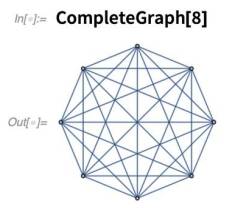
Each match corresponds to an edge in the graph:

And now by finding an “edge coloring” we have a list of possible “time slots” in which each match can be played:

EdgeChromaticNumber tells one the total number of matches needed:

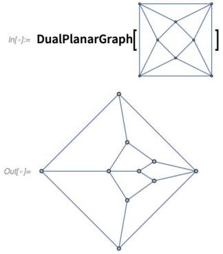
Map coloring brings up the subject of planar graphs. Version 13.0 introduces new functions for working with planar graphs. PlanarFaceList takes a planar graph and tells us how the graph can be decomposed into “faces”:

FindPlanarColoring directly computes a coloring for these planar faces. Meanwhile, DualPlanarGraph makes a graph in which each face is a vertex:

Subgraph Isomorphism & More

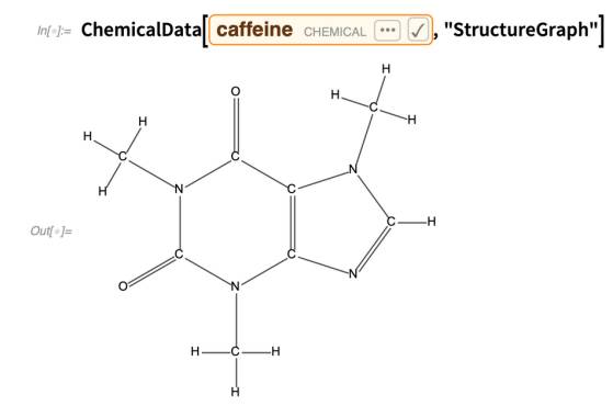
It comes up all over the place. (In fact, in our Physics Project it’s even something the universe is effectively doing throughout the network that represents space.) Where does a given graph contain a certain subgraph? In Version 13.0 there’s a function to determine that (the All says to give all instances):

A typical area where this kind of subgraph isomorphism comes up is in chemistry. Here is the graph structure for a molecule:

Now we can find a 6-cycle:

Now we can ask for the DominatorTreeGraph, which shows us a map of what vertices are critical to reach where, starting from A:

This now says for each vertex what its “dominator” is, i.e. what the nearest critical vertex to it is:

If the graph represents causal or other dependency of one “event” on others, the dominators are effectively synchronization points, where everything has to proceed through one “thread of history”.

Estimations of Spatial Fields

Imagine you’ve got data sampled at certain points in space, say on the surface of the Earth. The data might be from weather stations, soil samples, mineral drilling, or many other things. In Version 13.0 we’ve added a collection of functions for estimating “spatial fields” from samples (or what’s sometimes known as “kriging”).

Let’s take some sample data, and plot it:

Now let’s make a “spatial estimate” of the data:

This behaves much like an InterpolatingFunction, which we can sample anywhere we want:

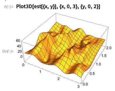
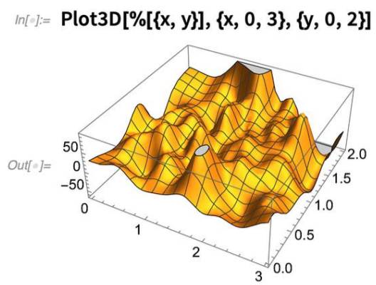
To create this estimate, we’ve inevitably used a model. We can change the model when we create the spatial estimate:

Now the results will be different:

In Version 13.0 you can get detailed control of the model by using options like SpatialTrendFunction and SpatialNoiseLevel. A key issue is what to assume about local variations in the spatial field—which you can specify in symbolic form using VariogramModel.

Getting Time Right: Leap Seconds & More

There are supposed to be exactly 24 hours in a day. Except that the Earth doesn’t know that. And in fact its rotation period varies slightly with time (generally its rotation is slowing down). So to keep the “time of day” aligned with where the Sun is in the sky the “hack” was invented of adding or subtracting “leap seconds”.

In a sense, the problem of describing a moment in time is a bit like the problem of geo location. In geo location there’s the question of describing a position in space. Knowing latitude-longitude on the Earth isn’t enough; one has to also have a “geo model” (defined by the GeoModel option) that describes what shape to assume for the Earth, and thus how lat-long should map to actual spatial position.

In describing a moment of time we similarly have to say how our “clock time” maps onto actual “physical time”. And to do that we’ve introduced in Version 13.0 the notion of a time system, defined by the TimeSystem option. This defines the first moment of December 2021 in the UT1 time system:

Here’s the first moment of December 2021 in the TAI time system:

But even though these are both associated with the same “clock description”, they correspond to different actual moments in time. And subtracting them we get a nonzero value:

What’s going on here? Well, TAI is a time system based on atomic clocks in which each day is taken to be precisely 24 hours long, and the “zero” of the time system was set in the late 1950s. UT1, on the other, is a time system in which each day has a length defined by the actual rotation of the Earth. And what this is showing is that in the time since TAI and UT1 were synchronized in the late 1950s the Earth’s actual rotation has slowed down to the point where it is now about 37 seconds behind where it would be with a precise 24-hour day. An important time system is UTC—which is standard “civil time”, and the de facto standard time of the internet. UTC doesn’t track the precise rotation speed of the Earth; instead it adds or subtracts discrete leap seconds when UT1 is about to accumulate another second of discrepancy from TAI—so that right now UTC is exactly 37 seconds behind TAI:

In Version 12.3 we introduced GeoOrientationData which is based on a feed of data on the measured rotation speed of the Earth. Based on this, here’s the deviation from 24 hours in the length of day for the past decade:

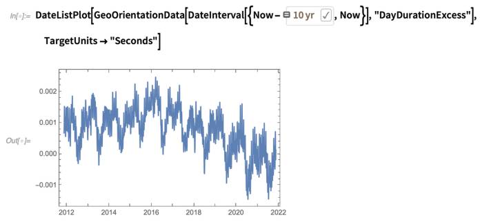
(And, yes, this shows that—for the first time since measurements were started in the late 1950s—the Earth’s rotation is slightly speeding up.)
Can we see the leap seconds that have been added to account for these changes? Let’s look at a few seconds right at the beginning of 2017 in the TAI time system:

Now let’s convert these moments in time into their UTC representation—using the new TimeSystemConvert function:

Look carefully at this. First, when 2016 ends and 2017 begins is slightly different in UTC than in TAI. But there’s something even weirder going on. At the very end of 2016, UTC shows a time 23:59:60. Why didn’t that “wrap around” in “clock arithmetic” style to the next day? Answer: because there’s a leap second being inserted. (Which makes me wonder just when the New Year was celebrated in time zone 0 that year….)

If you think this is subtle, consider another point. Inside your computer there are lots of timers that control system operations—and that are based on “global time”. And bad things could happen with these timers if global time “glitched”. So how can we address this? What we do in Wolfram Language is to use “smeared UTC”, and effectively smear out the leap second over the course of a day—essentially by making each individual “second” not exactly a “physical second” long.

Here’s the beginning of the last second of 2016 in UTC:

But here it is in smeared UTC:

And, yes, you can derive that number from the number of seconds in a “leapsecond day”:

By the way, you might be wondering why one should care about all this complexity. In everyday life leap seconds are a detail. But if you’re doing astronomy they can really matter. After all, in one (leap) second, light goes about 186,000 miles….

New, Crisper Geographic Maps

Maps involve a lot of data, and efficiently delivering them and rendering them (in appropriate projections, etc.) is a difficult matter. In Version 13.0 we’re greatly “crispening” maps, by using vector fonts for all labeling:

At least for right now, by default the background is still a bitmap. You can use “crispened” vector graphics for the background as well—but it will take longer to render:

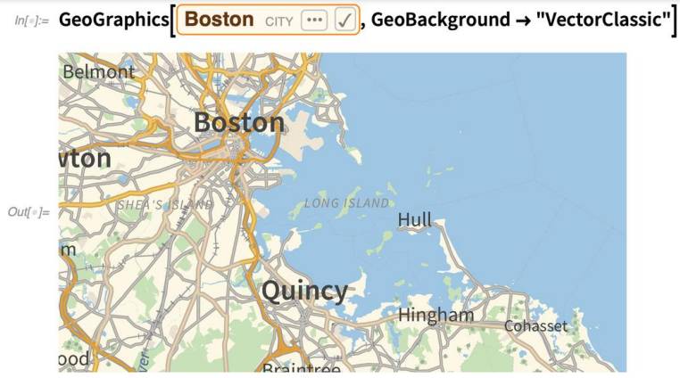
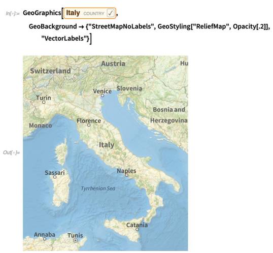
One advantage of using vector labels is that they can work in all geo projections (note that in Version 13 if you don’t specify the region for GeoGraphics, it’ll default to the whole world):

Another addition in Version 13 is the ability to mix multiple background layers. Here’s an example that includes a street map with a translucent relief map on top (and labels on top of that):

Geometric Regions: Fitting and Building

Given a bunch of points on a circle, what is the circle they are on? Here are random points selected around a circle:

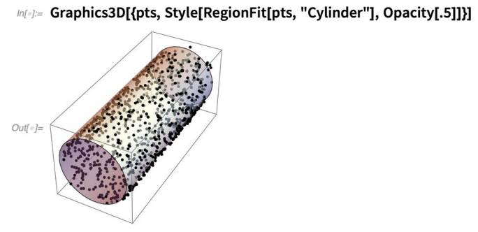
The new function RegionFit can figure out what circle the points are on:

Here’s a collection of points in 3D:

This fits a cylinder to these points:

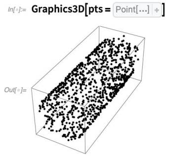
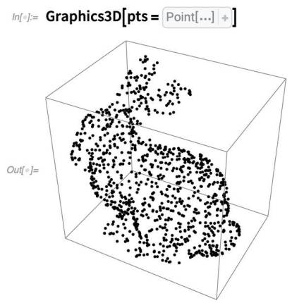
Another very useful new function in Version 13.0 is ConcaveHullMesh—which attempts to reconstruct a surface from a collection of 3D points. Here are 1000 points:

The convex hull will put “shrinkwrap” around everything:

But the concave hull will make the surface “go into the concavities”:

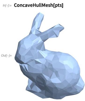
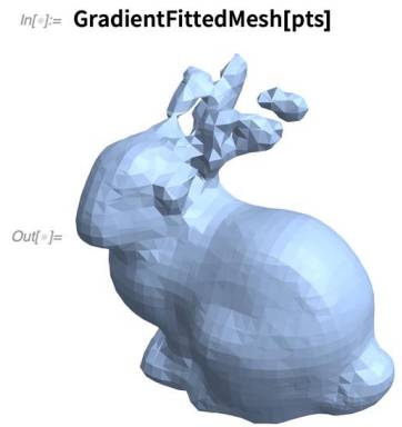
There’s a lot of freedom in how one can reconstruct the surface. Another function in Version 13 is GradientFittedMesh, which forms the surface from a collection of inferred surface normals:

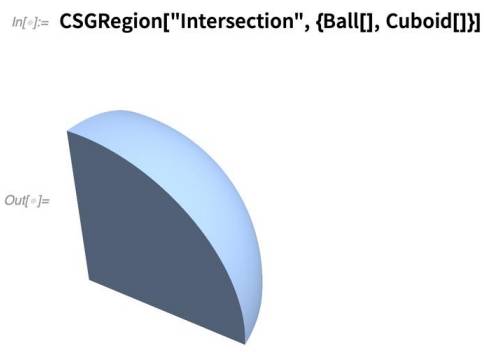
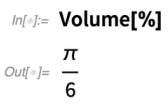
We’ve just talked about finding geometric regions from “point data”. Another new capability in Version 13.0 is constructive solid geometry (CSG), which explicitly builds up regions from geometric primitives. The main function is CSGRegion, which allows a variety of operations to be done on primitives. Here’s a region formed from an intersection of primitives:

Note that this is an “exact” region—no numerical approximation is involved. So when we ask for its volume, we get an exact result:

One can build up more complicated structures hierarchically:

Though the integrals get difficult, it’s still often possible to get exact results for things like volume:

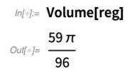
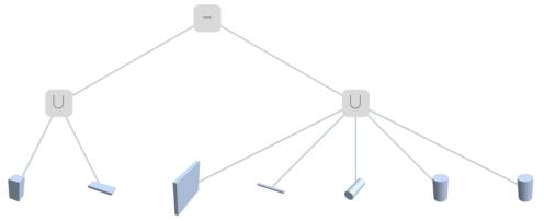
Given a hierarchically constructed geometric region, it’s possible to “tree it out” with CSGRegionTree:

In doing mechanical engineering, it’s very common to make parts by physically performing various operations that can easily be represented in CSG form. So here for example is a slightly more complicated CSG tree

which can be “assembled” into an actual CSG region for a typical engineering part:

Thinking about CSG highlights the question of determining when two regions are “the same”. For example, even though a region might be represented as a general Polygon, it may actually also be a pure Rectangle. And more than that, the region might be at a different place in space, with a different orientation. In Version 13.0 the function RegionCongruent tests for this:

RegionSimilar also allows regions to change size:

But knowing that two regions are similar, the next question might be: What transformation is needed to get from one to the other? In Version 13.0, FindRegionTransform tries to determine this:

Chemical Formulas & Chemical Reactions

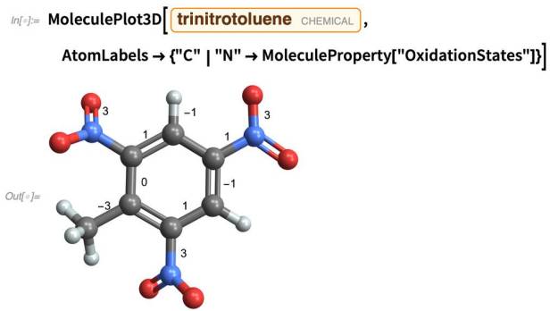
In Version 12 we introduced Molecule as a symbolic representation of a molecule in chemistry. In successive versions we’ve steadily been adding more capabilities around Molecule. In Version 13.0 we’re adding things like the capability to annotate 2D and 3D molecule plots with additional information:

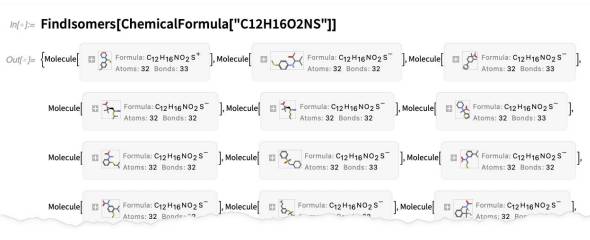
Molecule provides a representation for a specific type of molecule, with a specific arrangement of atoms in 3D space. In Version 13.0, however, we’re generalizing to arbitrary chemical formulas, in which one describes the number of each type of atom, without giving information on bonds or 3D arrangement. One can enter a chemical formula just as a string:

From the formula alone it’s possible to compute a few properties, like molecular mass:

Given the chemical formula, one can ask for specific “known” molecules that have that formula:

Often there will be many such molecules, and for example one could see how they’re arranged in “chemical feature space”:

Now that we can handle both molecules and chemical formulas, the next big step is chemical reactions. And in Version 13.0 the beginning of that is the ability to represent a chemical reaction symbolically.

You can enter a reaction as a string:

Here’s the reaction represented in terms of explicit rules:

But this is not yet a balanced reaction. To balance it, we can use ReactionBalance:

And, needless to say, ReactionBalance is quite general, so it can deal with reactions whose balancing requires solving slightly nontrivial Diophantine equations:

Bio Sequences: Plots, Secondary Bonds and
More

In Version 12.2 we introduced the concept of BioSequence, to represent molecules like DNA, RNA and proteins that consist of sequences of discrete units. In Version 13.0 we’re adding a variety of new BioSequence capabilities. One is BioSequencePlot, which provides an immediate visual representation of bio sequences:

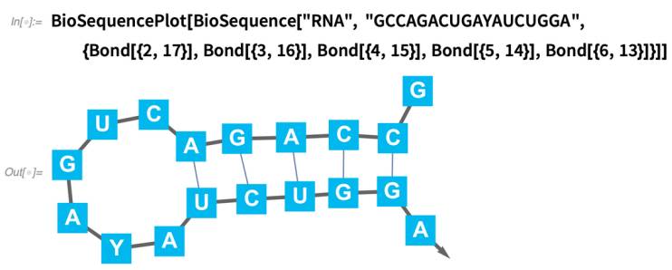
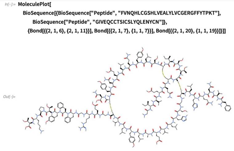
But beyond visualization, Version 13.0 also adds the ability to represent secondary structure in RNA, proteins and single-stranded DNA. Here, for example, is a piece of RNA with additional hydrogen bonds:

You can also specify secondary structure using “dot-bracket” notation:

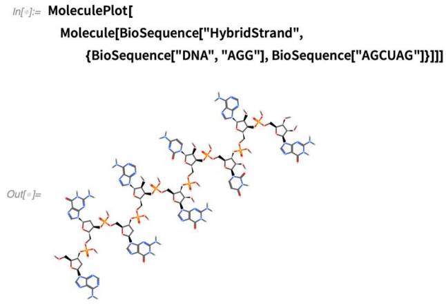
BioSequence also supports hybrid strands, involving for example linking between DNA and RNA:

Molecule converts BioSequence to an explicit collection of atoms:

Putting it all together, here’s an example of crosslinking between two peptides (now with disulfide bonds), in this case for insulin:

Flight Data

One of the goals of the Wolfram Language is to have as much knowledge about the world as possible. In Version 13.0 we’re adding a new domain: information about current and past airplane flights (for now, just in the US).
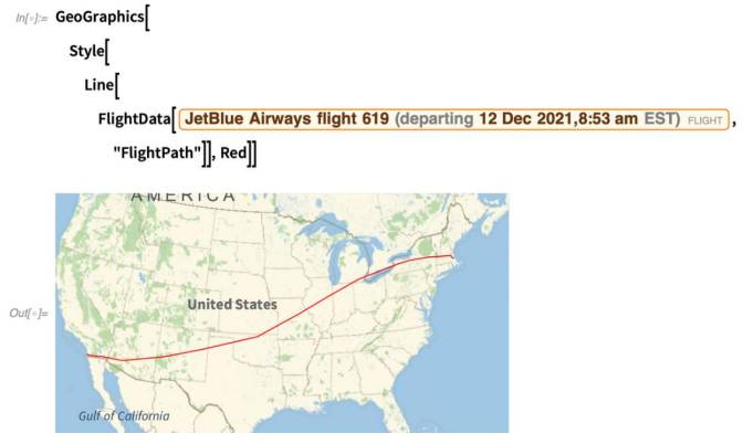
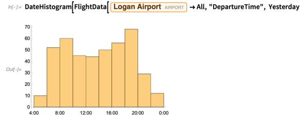
Let’s say we want to find out about flights between Boston and San Diego yesterday. We can just ask FlightData:

Now let’s look at one of those flights. It’s represented as a symbolic entity, with all sorts of properties:

This plots the altitude of the plane as a function of time:

And here is the flight path it followed:

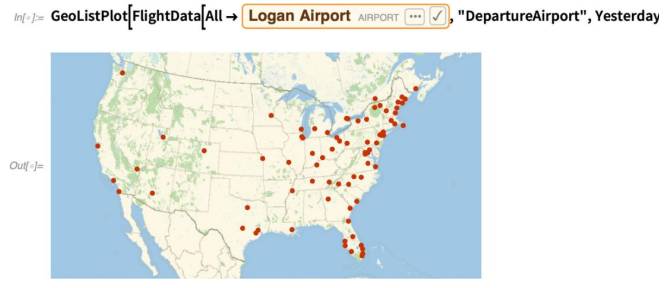
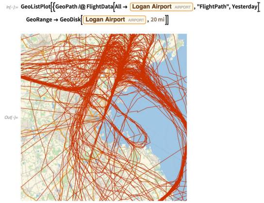
FlightData also lets us get aggregated data. For example, this tells where all flights that arrived yesterday in Boston came from:

And this shows a histogram of when flights departed from Boston yesterday:

Meanwhile, here are the paths flights arriving in Boston took near the airport:

And, yes, now one could start looking at the runway headings, wind directions yesterday, etc.—data for all of which we have in our knowledgebase.

Multiaxis and Multipanel Plots

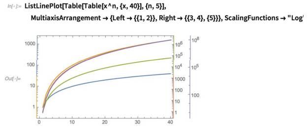
It’s been requested for ages. And there’ve been many package implementations of it. But now in Version 13.0 we have multiaxis plotting directly built into Wolfram Language. Here’s an example:

As indicated, the scale for the blue curve is on the left, and for the orange one on the right.

You might think this looks straightforward. But it’s not. In effect there are multiple coordinate systems all combined into one plot—and then disambiguated by axes linked by various forms of styling. The final step in the groundwork for this was laid in Version 12.3, when we introduced AxisObject and “disembodied axes”. Here’s a more complicated case, now with 5 curves, each with its own axis:

And here’s what happens if some curves share their axes:

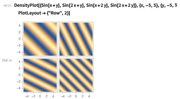
Multiple axes let you pack multiple curves onto a single “plot panel”. Multipanel plots let you put curves into separate, connected panels, with shared axes. The first cases of multipanel plots were already introduced in Version 12.0. But now in Version 13.0 we’re expanding multipanel plots to other types of visualizations:

Dates, and Infinities, in Plot Scales

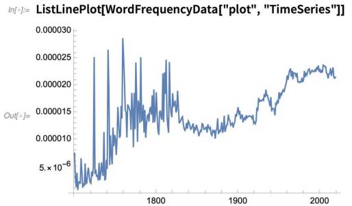
In Version 13.0, the “coordinates” in plots don’t just have to be numbers; they can be dates too. So for example this means that all the usual plotting functions “just work” on things like time series:

And there’s nothing stopping you having dates on multiple axes. Here’s an example of plotting time of day (a TimeObject) against date, in this case for email timestamps stored in a Databin:

Another thing that’s new with axes—or rather with scales—in Version 13.0 is the ability to have infinite plot ranges:

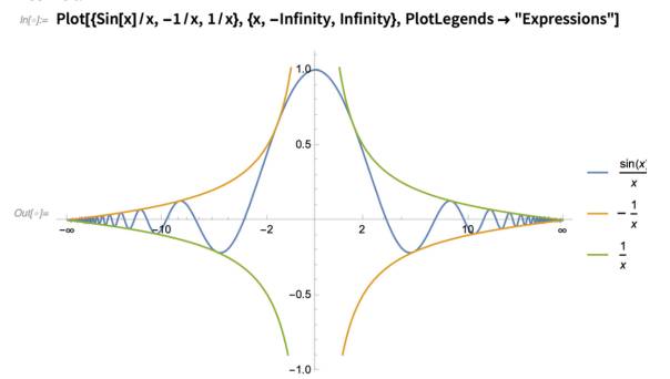
The way this works is that there’s a scaling function that maps the infinite interval to a finite one. You can use this explicitly with ScalingFunctions:

Here’s a slightly more elaborate example, that includes a doubly infinite interval:

New Visualization Types

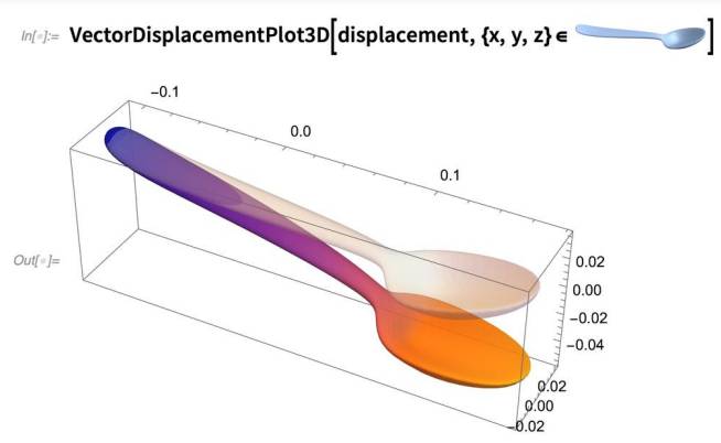
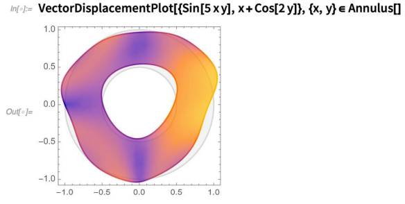
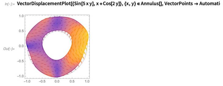
We’re constantly adding new types of built-in visualizations—not least to support new types of functionality. So, for example, in Version 13.0 we’re adding vector displacement plots to support our new capabilities in solid mechanics:

Or in 3D:

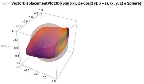
The plot shows how a given region is deformed by a certain displacement field. VectorPoints lets you include the displacement vectors as well:

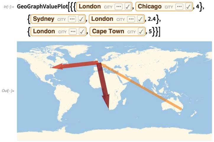
In Version 12.3 we introduced the function GeoGraphPlot for plotting graphs whose vertices are geo positions. In Version 13.0 we’re adding GeoGraphValuePlot which also allows you to visualize “values” on edges of the graph:

Lighting Goes Symbolic

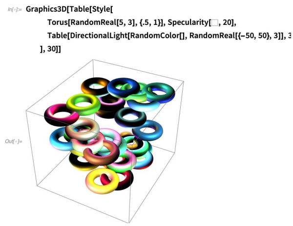
Lighting is a crucial element in the perception of 3D graphics. We’ve had the basic option Lighting for specifying overall lighting in 3D scenes ever since Version 1.0. But in Version 13.0 we’re making it possible to have much finer control of lighting—which has become particularly important now that we support material, surface and shading properties for 3D objects.
The key idea is to make the representation of light sources symbolic. So, for example, this represents a configuration of light sources which can immediately be used with the existing Lighting option:

But the new possibility is to “separately light” different objects in a scene, by specifying different symbolic “lighting styles” for them:

By the way, another new feature in Version 13.0 is the builtin Torus primitive:

Content Detectors for Machine Learning

Classify lets you train “whole data” classifiers. “Is this a cat?” or “Is this text about movies?” In Version 13.0 we’ve added the capability to train content detectors that serve as classifiers for subparts of data. “What cats are in here?” “Where does it talk about movies here?” The basic idea is to give examples of whole inputs, in each case saying where in the input corresponds to a particular class. Here’s some basic training for picking out classes of topics in text:

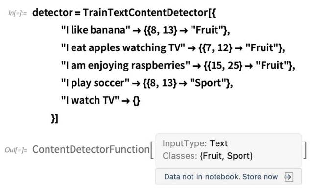
Now we can use the content detector on specific inputs:

How does this work? Basically what’s happening is that the Wolfram Language already knows a great deal about text and words and meanings. So you can just give it an example that involves soccer, and it can figure out from its built-in knowledge that basketball is the same kind of thing.

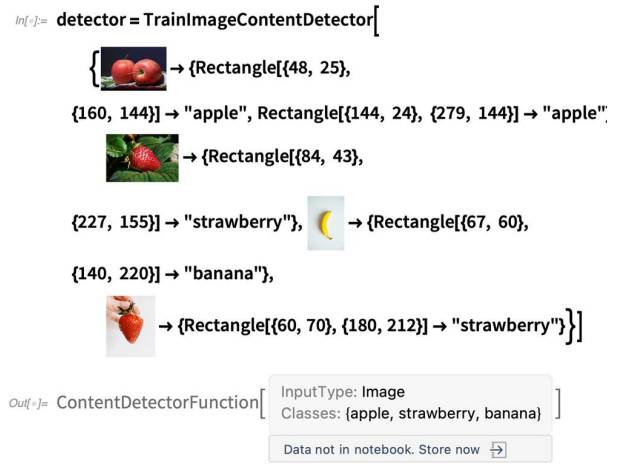
In Version 13.0 you can create content detectors not just for text but also for images. The problem is considerably more complicated for images, so it takes longer to build the content detector. Once built, though, it can run rapidly on any image.

Just like for text, you train an image content detector by giving sample images, and saying where in those images the classes of things you want occur:

Having done this training (which, yes, took about 5 minutes on a GPUenabled machine), we can then apply the detector we just created:

When you apply the detector, you can ask it for various kinds of information. Here it’s giving bounding boxes that you can use to annotate the original image:

By the way, what’s happening under the hood to make all of this work is quite sophisticated. Ultimately we’re using lots of built-in knowledge about the kinds of images that typically occur. And when you supply sample images we’re augmenting these with all kinds of “typical similar” images derived by transforming your samples. And then we’re effectively retraining our image system to make use of the new information derived from your examples.

New Visualization & Diagnostics for Machine
Learning

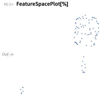
One of the machine learning–enabled functions that I, for one, use all the time is FeatureSpacePlot. And in Version 13.0 we’re adding a new default method that makes FeatureSpacePlot faster and more robust, and makes it often produce more compelling results. Here’s an example of it running on 10,000 images:

One of the great things about machine learning in the Wolfram Language is that you can use it in a highly automated way. You just give Classify a collection of training examples, and it’ll automatically produce a classifier that you can immediately use. But how exactly did it do that? A key part of the pipeline is figuring out how to extract features to turn your data into arrays of numbers. And in Version 13.0 you can now get the explicit feature extractor that’s been constructed for (so you can, for example, use it on other data):

Here are the extracted features for a single piece of data:

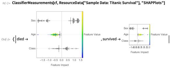
This shows some of the innards of what’s happening in Classify. But another thing you can do is to ask what most affects the output that Classify gives. And one approach to this is to use SHAP values to determine the impact that each attribute specified in whatever data you supply has on the output. In Version 13.0 we’ve added a convenient graphical way to display this for a given input:

Automating the Problem of Tracking for Robots and More

Designing control systems is a complicated matter. First, you have to have a model for the system you’re trying to control. Then you have to define the objectives for the controller. And then you have to actually construct a controller that achieves those objectives. With the whole stack of technology in Wolfram Language and Wolfram System Modeler we’re getting to the point where we have an unprecedentedly automated pipeline for doing these things. Version 13.0 specifically adds capabilities for designing controllers that make a system track a specified signal—for example having a robot that
follows a particular trajectory. Let’s consider a very simple robot that consists of a moving cart with a pointer attached:

First, we need a model for the robot, and this we can create in Wolfram System Modeler (or import as a Modelica model):

Our goal now is to set up a way to “drive” the input variables for the robot (the force moving the cart, and the torque for the pointer)

in order to achieve certain behavior for the output variables (the position of the end of the pointer):

Here’s a curve that we want the end of the pointer to follow over time:

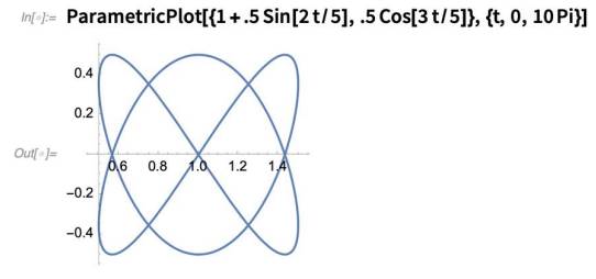
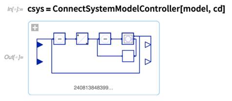
Now we want to actually construct the controller—and this is where one needs to know a certain amount about control theory. Here we’re going to use the method of pole placement to create our controller. And we’re going to use the new capability of Version 13.0 to be able to design a “tracking controller” that tracks specified outputs (yes, to set those numbers you have to know about control theory):

Now we have to make the closed-loop system that includes the robot and its controller:

And now we can simulate the behavior of this whole system, giving lists of the x and y coordinates of the reference trajectory as input:

And based on this simulation here’s a plot of where the end of the pointer goes:

After an initial transient, this follows the path we wanted. And, yes, even though this is all a bit complicated, it’s unbelievably simpler than it would be if we were directly using real hardware, rather than doing theoretical “model-based” design.

Type Fewer Brackets!

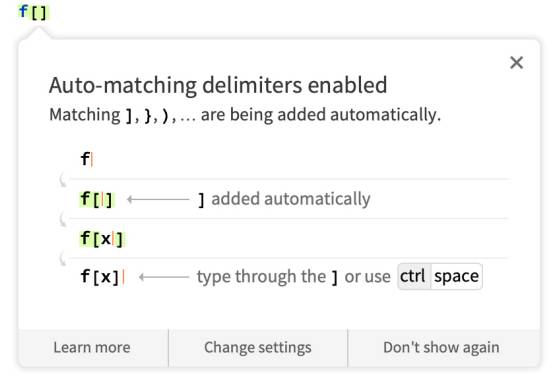
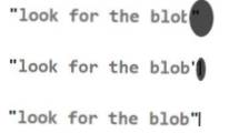
When you first launch Version 13, and you type something like f[ you’ll see the following:

What Version 13 is now doing is to automatically add matching brackets when it thinks it’s unambiguous to do so. The one thing to learn is that you can then “type through” the bracket; in other words if this case with the cursor right before the auto-added ] you explicitly type ] then no new ] will appear; the system will just “type through” the ]. There’s also the alternative of using ctrlspace to move to the right of the auto-added closing bracket. And, by the way, ctrlspace also “moves to the right” of the next closing bracket even when your cursor isn’t immediately next to the bracket; it’ll do this even if the cursor is deep inside a nested structure.

The automatching behavior (which you can turn off in the Preferences dialog if you really don’t like it) applies not only to [ ] but also to { }, ( ), [[ ]], <| |>, (* *) and (importantly) ” “. And ctrlspace also works with all these kinds of delimiters. For serious user-experience aficionados there’s an additional point perhaps of interest. Typing ctrlspace can potentially move your cursor sufficiently far that your eye loses it. This kind of long-range cursor motion can also happen when you enter math and other 2D material that is being typeset in real time. And in the 1990s we invented a mechanism to avoid people “losing the cursor”. Internally we call it the “incredible shrinking blob”. It’s a big black blob that appears at the new position of the cursor, and shrinks down to the pure cursor in about 160 milliseconds. Think of this as a “vision hack”. Basically we’re plugging into the human pre-attentive vision system, that causes one to automatically shift one’s gaze to the “suddenly appearing object”, but without really noticing one’s done this. In Version 13 we’re now using this mechanism not just for real-time typesetting, but also for ctrlspace—adding the blob whenever the “jump distance” is above a certain threshold. You’ll probably not even notice that the blob is there (only a small fraction of people seem to “see” it). But if you catch it in time, here’s what you’ll see:

Progress in Seeing the Progress of Computations…

You’re running a long computation. What’s going on with it? We have a long-term initiative to provide interactive progress monitoring for as many functions that do long computations as possible.

An example in Version 13.0 is that ParallelMap, ParallelTable, etc. automatically give you progress monitoring:

The display is temporary; it’s only there while the computation is running, and then it goes away.
There are many other examples of this, and more to come. There’s progress monitoring in video, machine learning, knowledgebase access, import/export and various algorithmic functions:

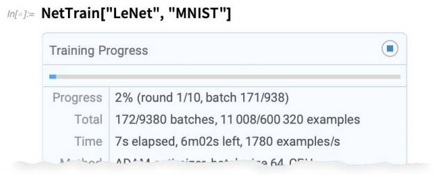
Generally, progress monitoring is just a good thing; it helps you know what’s happening, and allows you to check if things have gone off track. But sometimes it might be confusing, especially if there’s some inner function that you didn’t even know was being called—and you suddenly see progress monitoring for it. For a long time we had thought that this issue would make widespread progress monitoring a bad idea. But the value of seeing what’s going on seems to almost always outweigh the potential confusion of seeing something happening “under the hood” that you didn’t know about. And it really helps that as soon as some operation is over, its progress monitors just disappear, so in your final notebook there’s no sign of them.

By the way, each function with progress monitoring has a ProgressReporting option, which you can set to False. In addition, there is a global variable $ProgressReporting which specifies the default throughout the system.

It’s worth mentioning that there are different levels of “Are we there yet?” monitoring that can be given. Some functions go through a systematic sequence of steps, say processing each frame in a video. And in such cases it’s possible to show the “fraction complete” as a progress indicator bar. Sometimes it’s also possible to make at least some guess about the “fraction complete” (and therefore the expected completion time) by looking “statistically” at what’s happened in parts of the computation so far. And this is, for example, how ParallelMap etc. do their progress monitoring. Of course, in general it’s not possible to know It’s worth mentioning that there are different levels of “Are we there yet?” monitoring that can be given. Some functions go through a systematic sequence of steps, say processing each frame in a video. And in such cases it’s possible to show the “fraction complete” as a progress indicator bar. Sometimes it’s also possible to make at least some guess about the “fraction complete” (and therefore the expected completion time) by looking “statistically” at what’s happened in parts of the computation so far. And this is, for example, how ParallelMap etc. do their progress monitoring. Of course, in general it’s not possible to know how long an arbitrary computation will take; that’s the story of
computational irreducibility and things like the undecidability of the halting problem for Turing machines. But with the assumption (that turns out to be pretty good most of the time) that there’s a fairly smooth distribution of running times for different subcomputations, it’s still possible to give reasonable estimates. (And, yes, the “visible sign” of potential undecidability is that a percentage complete might jump down as well as going up with time.)

Wolfram| Alpha Notebooks

For many years we had Mathematica + Wolfram Language, and we had Wolfram|Alpha. Then in late 2019 we introduced Wolfram|Alpha Notebook Edition as a kind of blend between the two. And in fact in standard desktop and cloud deployments of Mathematica and Wolfram|Alpha there’s also now the concept of a Wolfram|Alpha-Mode Notebook, where the basic idea is that you can enter things in free-form natural language, but get the capabilities of Wolfram Language in representing and building up computations:

In Version 13.0 quite a lot has been added to Wolfram|Alpha-Mode Notebooks. First, there are palettes for directly entering 2D math notation:

There’s also now the capability to immediately generate rich dynamic content directly from free-form linguistic input:

In addition to “bespoke” interactive content, in Wolfram|Alpha-Mode Notebooks one can also immediately access interactive content from the 12,000+ Demonstrations in the Wolfram Demonstrations Project:

Wolfram|Alpha Notebook Edition is particularly strong for education. And in Version 13.0 we’re including a first collection of interactive quizzes, specifically about plots:

Everything for Quizzes TRight in the Language

Version 13.0 introduces the ability to create, deploy and grade quizzes directly in Wolfram Language, both on the desktop and in the cloud. Here’s an example of a deployed quiz:

How was this made? There’s an authoring notebook, that looks like this:

It’s all based on the form notebook capabilities that we introduced in Version 12.2. But there’s one additional element: QuestionObject. A QuestionObject gives a symbolic representation of a question to ask, together with an AssessmentFunction to apply to the answer that’s provided, to assess, grade or otherwise process it.In the simplest case, the “question to ask” is just a string. But it can be more sophisticated, and there’s a list of possibilities (that will steadily grow) that you can select in the authoring notebook:

(The construct QuestionInterface lets you control in detail how the “question prompt” is set up.)
Once you’ve created your quiz in the authoring notebook (and of course it doesn’t need to be just a “quiz” in the courseware sense), you need to deploy it. Settings allow you to set various options:

Then when you press Generate you immediately get a deployed version of your quiz that can, for example, be accessed directly on the web. You also get a results notebook, that shows you how to retrieve results from people doing the quiz.

So what actually happens when someone does the quiz? Whenever they press Submit their answer will be assessed and submitted to the destination you’ve specified—which can be a cloud object, a databin,
etc. (You can also specify that you want local feedback given to the person who’s doing the quiz.)
So after several people have submitted answers, here’s what the results you get might look like:

All in all, Version 13.0 now provides a streamlined workflow for creating both simple and complex quizzes. The quizzes can involve all sorts of different types of responses—notably including runnable Wolfram Language code. And the assessments can also be sophisticated—for example including code comparisons. Just to give a sense of what’s possible, here’s a question that asks for a color to be selected, that will be compared with the correct answer to within some tolerance:

Untangling Email, BPDFs and More

What do email threads really look like? I’ve wondered this for ages. And now in Version 13.0 we have an easy way to import MBOX files and see the threading structure of email. Here’s an example from an internal mailing list of ours:

Now we can do standard graph operations on this:

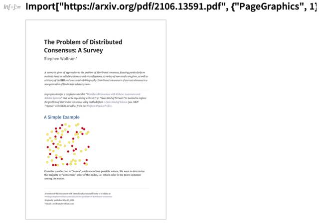
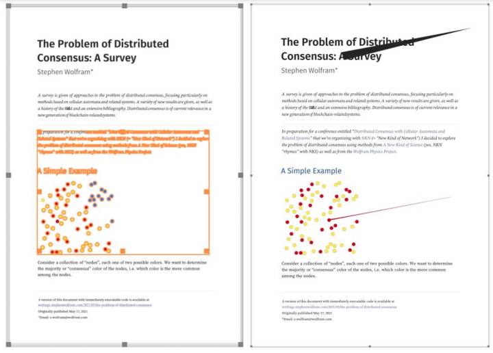
An important new feature of Version 12.2 was the ability to faithfully import PDFs in a variety of forms—including page images and plain text. In Version 13.0 we’re adding the capability to import PDFs as vector graphics.

Here’s an example of pages imported as images:

Now here’s a page imported as vector graphics:

And now, to prove it’s vector graphics, we can actually go in and modify it, right down to the strokes used in each glyph:

Now that we have Video in Wolfram Language, we want to be able to import as many videos as possible. We already support a very complete list of video containers and codecs. In Version 13.0 we’re also adding the ability to import .FLV (Flash) videos, giving you the opportunity to convert them to modern formats.

CloudExpression Goes Mainstream

You’ve got an expression you want to manipulate across sessions. One way to do this is to make the whole expression persistent using PersistentValue—or explicitly store it in a file or a cloud object and read it back when you need it. But there’s a much more efficient and seamless way to do this—that doesn’t require you to deal with the whole expression all the time, but instead lets you “poke” and “peek” at individual parts—and that’s to use CloudExpression.

We first introduced CloudExpression back in 2016 in Version 10.4. At that time it was intended to be a fairly temporary way to store fairly small expressions. But we’ve found that it’s a lot more generally useful than we expected, and so in Version 13.0 it’s getting a major upgrade that makes it more efficient and robust.

It’s worth mentioning that there are several other ways to store things persistently in the Wolfram Language. You can use PersistentValue to persist whole expressions. You can use Wolfram Data Drop functionality to let you progressively add to databins. You can use ExternalStorageUpload to store things in external storage systems like S3 or IPFS. Or you can set up an external database (like an SQL- or document-based one), and then use Wolfram Language functions to access and update this.

But CloudExpression provides a much more lightweight, yet general, way to set up and manipulate persistent expressions. The basic idea is to create a cloud expression that is stored persistently in your cloud account, and then to be able to do operations on that expression. If the cloud expression consists of lists and associations, then standard Wolfram Language operations let you efficiently read or write parts of the cloud expression without ever having to pull the whole thing into
memory in your session.

This creates a cloud expression from a table of, in this case, polynomials:

This gives us the 5th part of the table:

We can reset it:

This gets the whole cloud expression:

But the important point is that getting and setting parts of the cloud expression don’t require pulling the expression into memory. Each operation is instead done directly in the cloud.

In a traditional relational database system, there’d have to be a certain “rectangularity” to the data. But in a cloud expression (like in a NoSQL database) you can have any nested list and association structure, and, in addition, the elements can be arbitrary symbolic expressions. CloudExpression is set up so that operations you use are atomic, so that, for example, you can safely have two different processes concurrently reading and writing to the same cloud expression. The result is that CloudExpression is a good way to handle data built up by things like APIFunction and FormFunction. By the way, CloudExpression is ultimately in effect just a cloud object, so it shares permission capabilities with CloudObject. And this means, for example, that you can let other people read—or write—to a cloud expression you created. (The data associated with CloudExpression is stored in your cloud account, though it uses its own storage quota, separate from the one for CloudObject.) Let’s say you store lots of important data as a sublist in CloudExpression. CloudExpression is so easy to use, you might worry that you’d just type something like ce[“customers”]=7 and suddenly your critical data would be overwritten. To avoid this, CloudExpression has the option PartProtection, which allows you to specify whether, for example, you want to allow the structure of the expression to be changed, or only its “leaf elements”.

The Advance of the Function Repository

When we launched the Wolfram Function Repository in 2019 we didn’t know how rapidly it would grow. But I’m happy to say that it’s been a great success—with perhaps 3 new functions per day being published, giving a total to date of 2259 functions. These are functions which are not part of the core Wolfram Language, but can immediately be accessed from any Wolfram Language system.

They are functions contributed by members of the community, and reviewed and curated by us. And given all of the capabilities of the core Wolfram Language it’s remarkable what can be achieved in a single contributed function. The functions mostly don’t have the full breadth and robustness that would be needed for integration into the core Wolfram Language (though functions like Adjugate in Version 13.0 were developed from “prototypes” in the Function Repository). But what they have is a greatly accelerated delivery process which allows convenient new functionality in new areas to be made available extremely quickly. Some of the functions in the Function Repository extend algorithmic capabilities. An example is FractionalOrderD for computing fractional derivatives:

There’s a lot in FractionalOrderD. But it’s in a way quite specific—in the sense that it’s based on one particular kind of fractional differentiation. In the future we may build into the system full-scale fractional differentiation, but this requires a host of new algorithms. What FractionalOrderD in the Function Repository does is to deliver one form of fractional differentiation now. Here’s another example of a function in the Function Repository, this time one that’s based on capabilities in Wolfram|Alpha:

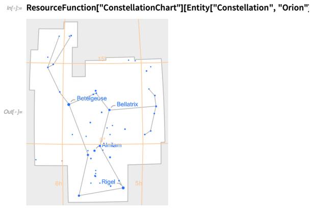
Some functions provide extended visualization capabilities. Here’s VennDiagram:

There are many ways to imagine handling more complicated cases; this function makes a particular choice:

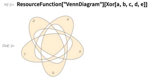
As another example of a visualization function, here’s TruthTable—built to give a visual display of the results of the core language BooleanTable function:

Some functions give convenient—though perhaps not entirely general—extensions to particular features of the language.

Here’s IntegerChop that reduces real numbers “sufficiently close to integers” to exact integers:

Here’s an example of a function that perhaps one day will be in the core language. But for now the most common cases of it are provided by a Function Repository function:

There are lots of functions in the Function Repository that give specific extensions to areas of functionality in the core language. BootstrappedEstimate, for example, gives a useful, specific extension to statistics functionality:

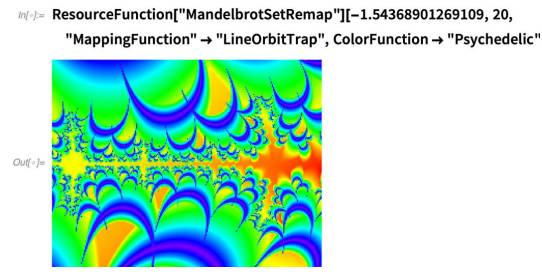
Here’s a function that “remaps” the Mandelbrot set— using FunctionCompile to go further than MandelbrotSetPlot:

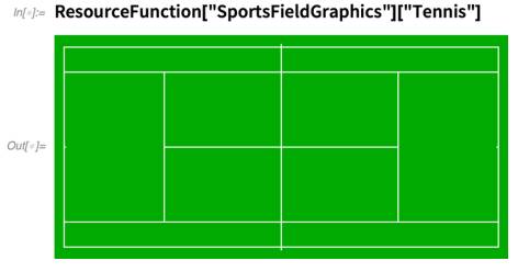
There are some functions that definitely seem “niche”—but are extremely useful if you need them:

Then there are functions that make “current issues” convenient. An example is MintNFT:

There are also “functions for fun” (that can definitely also be useful):

And there are functions that might be considered “insider” humor:

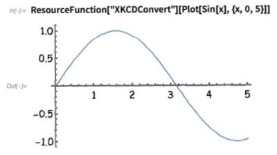
By the way, it’s not just the Function Repository that’s been growing with all sorts of great contributions: there’s also the Data Repository and Neural Net Repository, which have also been energetically advancing.

Introducing Tools for the Creation of Paclets

The Function Repository is all about creating single functions that add functionality. But what if you want to create a whole new world of functionality, with many interlinked functions? And perhaps one that also involves not just functions, but for example changes to elements of your user interface too. For many years we’ve internally built many parts of the Wolfram Language system using a technology we call paclets—that effectively deliver bundles of functionality that can get automatically installed on any given user’s system. In Version 12.1 we opened up the paclet system, providing specific functions like PacletFind and PacletInstall for using paclets. But creating paclets was still something of a black art. In Version 13.0 we’re now releasing a first round of tools to create paclets, and to allow you to deploy them for distribution as files or through the Wolfram Cloud. The paclet tools are themselves (needless to say) distributed in a paclet that is now included by default in every Wolfram Language installation. For now, the tools are in a separate package that you have to load:

To begin creating a paclet, you define a “paclet folder” that will contain all the files that make up your paclet:

This sets up the basic outline structure of your paclet, which you can then add files to:

As an alternative, you could specify some components in your paclet right when you first create the paclet:

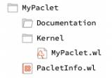
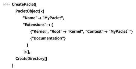
There are all sorts of elements that can exist in paclets, and in future versions there’ll be progressively more tooling to make it easier to create them. In Version 13.0, however, a major piece of tooling that is
being delivered is Documentation Tools, which provides tools for creating the same kind of documentation that we have for built-in system functions.
You can access these tools directly from the main system Palettes menu:

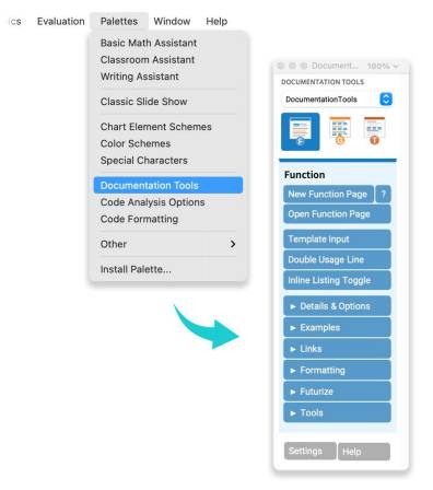
Now you can create as notebooks in your paclet function reference pages, guide pages, tech notes and other documentation elements. Once you’ve got these, you can build them into finished documentation using PacletDocumentationBuild. Then you can have them as notebook files, standalone HTML files, or deployed material in the cloud.

Coming soon will be additional tools for paclet creation, as well as a public Paclet Repository for user-contributed paclets. An important feature to support the Paclet Repository—and that can already be used with privately deployed paclets—is the new function PacletSymbol. For the Function Repository you can use ResourceFunction[“name”] to access any function in the repository. PacletSymbol is an analog of this for paclets. One way to use a paclet is to explicitly load all its assets. But PacletSymbol allows you to “deep call” into a paclet to access a single function or symbol. Just like with ResourceFunction, behind the scenes all sorts of loading of assets will still happen, but in your code you can just use PacletSymbol without any visible initialization. And, by the way, an emerging pattern is to “back” a collection of interdependent Function Repository functions with a paclet, accessing the individual functions from the code in the Function Repository using PacletSymbol.

Introducing Context Aliases

When you use a name, like x, for something, there’s always a question of “which x?” From the very beginning in Version 1.0 there’s always been the notion of a context for every symbol. By default you create symbols in the Global context, so the full name for the x you make is Global`x. When you create packages, you typically want to set them up so the names they introduce don’t interfere with other names you’re using. And to achieve this, it’s typical to have packages define their own contexts. You can then always refer to a symbol within a package by its full name, say Package`Subpackage`x etc.

But when you just ask for x, what do you get? That’s defined by the setting for $Context and $ContextPath.

But sometimes you want an intermediate case. Rather than having just x represent Package`x as it would if Package` were on the context path $ContextPath, you want to be able to refer to x “in its package”, but without typing (or having to see) the potential long name of its package. In Version 13.0 we’re introducing the notion of context aliases to let you do this. The basic idea is extremely simple. When you do Needs[“Context`”] to load the package defining a particular context, you can add a “context alias”, by doing Needs[“Context`”->”alias`”]. And the result of this will be that you can refer to any symbol in that context as alias`name. If you don’t specify a context alias, Needs will add the context you ask for to $ContextPath so its symbols will be available in
“just x” form. But if you’re working with many different contexts that could have symbols with overlapping names, it’s a better idea to use context aliases for each context. If you define short aliases there won’t be much more typing, but you’ll be sure to always refer to the correct symbol.

This loads a package corresponding to the context ComputerArithmetic`, and by default adds that context to $ContextPath:

Now symbols with ComputerArithmetic can be used without saying anything about their context:

This loads the package defining a context alias for it:

Now you can refer to its symbols using the alias:

The global symbol $ContextAliases specifies all the aliases that you currently have in use:

By the way, just like our convention about symbols having names that start with uppercase letters, it’s been a common general convention to have context names for packages also start with uppercase letters. Now that we have context aliases as well, we’re suggesting the convention of using lowercase letters for these.

Symbolic Webpage Construction

If you want to take a notebook and turn it into a webpage, all you need do is CloudPublish it. Similarly, if you want to create a form on the web, you can just use CloudPublish with FormFunction (or FormPage). And there are a variety of other direct-to-web capabilities that have long been built into the Wolfram Language.

But what if you want to make a webpage with elaborate web elements? One way is to use XMLTemplate to insert Wolfram Language output into a file of HTML etc. But in Version 13.0 we’re beginning the process of setting up symbolic specifications of full webpage structure, that let you get the best of both Wolfram Language and web capabilities and frameworks.

Here’s a very small example:

And here’s the webpage it produces:

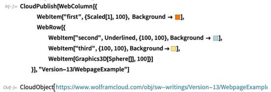
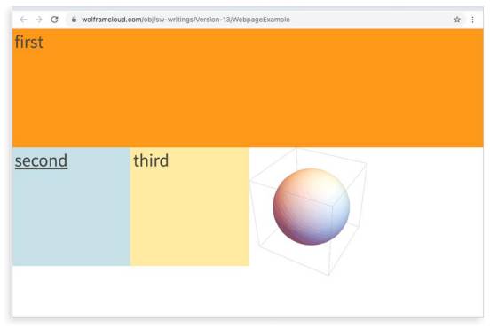
The basic idea is to construct webpages using nested combinations of WebColumn, WebRow and WebItem. Each of these have various Wolfram Language options. But they also allow direct access to CSS options. So in addition to a Wolfram Language Background->LightBlue option, you can also use a CSS option like “border-right”->”1px solid #ddd”.

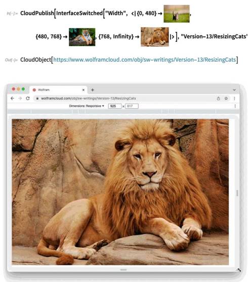
There’s one additional critical feature: InterfaceSwitched. This is the core of being able to create responsive webpages that can change their structure when viewed on different kinds of devices. InterfaceSwitched is a symbolic construct that you can insert anywhere inside WebItem, WebColumn, etc. and that can behave differently when accessed with a different interface. So, for example will behave as 1 if it’s accessed from a device with a width between 0 and 480 pixels, and so on. You can see this in action using CloudPublish

and then just resizing the window you use to view the result:

And Now… NFTs!

One of the things that’s happened in the world since the release of Version 12.3 is the mainstreaming of the idea of NFTs. We’ve actually had tools for several years for supporting NFTs—and tokens in general—on blockchains. But in Version 13.0 we’ve added more streamlined NFT tools, particularly in the context of our connection to the Cardano blockchain.

The basic idea of an NFT (“non-fungible token”) is to have a unique token that can be transferred between users but not replicated. It’s like a coin, but every NFT can be unique. The blockchain provides a permanent ledger of who owns what NFT. When you transfer an NFT what you’re doing is just adding something to the blockchain to record that transaction.

What can NFTs be used for? Lots of things. For example, we issued “NFT certificates” for people who “graduated” from our Summer School and Summer Camp this year. We also issued NFTs to record ownership for some cellular automaton artworks we created in a livestream. And in general NFTs can be used as permanent records for anything: ownership, credentials or just a commemoration of an achievement or event.

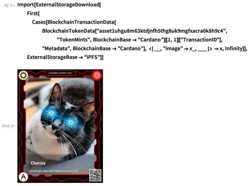
In a typical case, there’s a small “payload” for the NFT that goes directly on the blockchain. If there are larger assets—like images—these will get stored on some distributed storage system like IPFS, and the payload on the blockchain will contain a pointer to them. Here’s an example that uses several of our blockchain functions—as well as the new connection to the Cardano blockchain—to retrieve from IPFS the image associated with an NFT that we minted a few weeks ago:

How can you mint such an NFT yourself? The Wolfram Language has the tools to do it. ResourceFunction[“MintNFT“] in the Wolfram Function Repository provides one common workflow (specifically for the CIP 25 Cardano NFT standard)—and there’ll be more coming.
The full story of blockchain below the “pure consumer” level is complicated and technical. But the Wolfram Language provides a
uniquely streamlined way to handle it, based on symbolic representations of blockchain constructs, that can directly be manipulated using all the standard functions of the Wolfram Language. There are also many different blockchains, with different setups. But through lots of effort that we’ve made in the past few years, we’ve been able to create a uniform framework that interoperates between different blockchains while still allowing access to all of their special features. So now you just set a different BlockchainBase (Bitcoin, Ethereum, Cardano, Tezos, ARK, Bloxberg, …) and you’re ready to
interact with a different blockchain.

Sleeker, Faster Downloading

Everything I’ve talked about here is immediately available today in the Wolfram Cloud and on the desktop—for macOS, Windows and Linux (and for the macOS, that’s both Intel and “Apple Silicon” ARM). But when you go to download (at least for macOS and Windows) there’s a new option: download without local documentation. The actual executable package that is Wolfram Desktop or Mathematica is about 1.6 GB for Windows and 2.1 GB for macOS (it’s bigger for macOS because it includes “universal” binaries that cover both Intel and ARM). But then there’s documentation. And there’s a lot of it. And if you download it all, it’s another 4.5 GB to download, and 7.7 GB when deployed on your system. The fact that all this documentation exists is very important, and we’re proud of the breadth and depth of it. And it’s definitely convenient to have this documentation right on your computer—as notebooks that you can immediately bring up, and edit if you want. But as our documentation has become larger (and we’re working on making it even larger still) it’s sometimes a better optimization to save the local space on your computer, and instead get documentation from the web. So in Version 13.0 we’re introducing documentationless downloads— which just go to the web and display documentation in your browser. When you first install Mathematica or Wolfram|One you can choose the “full bundle” including local documentation. Or you can choose to install only the executable package, without documentation. If you change your mind later, you can always download and install the documentation using the Install Local Documentation item in the Help menu.

(By the way, the Wolfram Engine has always been documentationless— and on Linux its download size is just 1.3 GB, which I consider incredibly small given all its functionality.)

Mathematica V13